
Piotr Ptak
AIRCRAFT TRACKING AND CLASSIFICATION WITH
VHF PASSIVE BISTATIC RADAR
Acta Universitatis
Lappeenrantaensis 647
Thesis for the degree of Doctor of Science (Technology) to be presented with
due permission for public examination and criticism in Auditorium 1383 at
Lappeenranta University of Technology, Lappeenranta, Finland on the 25th of
June, 2015, at 12 pm.

Supervisor
Docent, PhD Tuomo Kauranne
Faculty of Technology
Department of Mathematics and Physics
Lappeenranta University of Technology
Finland
Reviewers
Prof. Pekka Neittaanmäki
Department of Mathematical Information Technology
University of Jyväskylä
Finland
PhD Hannu-Heikki Puupponen
Department of Mathematical Information Technology
University of Jyväskylä
Finland
Opponent
Prof. Pekka Neittaanmäki
Department of Mathematical Information Technology
University of Jyväskylä
Finland
ISBN 978-952-265-815-9
ISBN 978-952-265-816-6 (PDF)
ISSN-L 1456-4491
ISSN 1456-4491
Lappeenrannan teknillinen yliopisto
Yliopistopaino 2015

Abstract
Piotr Ptak
AIRCRAFT TRACKING AND CLASSIFICATION WITH VHF PASSIVE BISTATIC RADAR
Lappeenranta, 2015
118 p.
Acta Universitatis Lappeenrantaensis 647
Diss. Lappeenranta University of Technology
ISBN 978-952-265-815-9, ISBN 978-952-265-816-6 (PDF), ISSN-L 1456-4491, ISSN 1456-4491
Since the times preceding the Second World War the subject of aircraft tracking has been a core in-
terest to both military and non-military aviation. During subsequent years both technology and con-
figuration of the radars allowed the users to deploy it in numerous fields, such as over-the-horizon
radar, ballistic missile early warning systems or forward scatter fences. The latter one was arranged
in a bistatic configuration. The bistatic radar has continuously re-emerged over the last eighty years
for its intriguing capabilities and challenging configuration and formulation. The bistatic radar ar-
rangement is used as the basis of all the analyzes presented in this work.
The aircraft tracking method of VHF Doppler-only information, developed in the first part of this
study, is solely based on Doppler frequency readings in relation to time instances of their appear-
ance. The corresponding inverse problem is solved by utilising a multistatic radar scenario with
two receivers and one transmitter and using their frequency readings as a base for aircraft trajectory
estimation. The quality of the resulting trajectory is then compared with ground-truth information
based on ADS-B data.
The second part of the study deals with the developement of a method for instantaneous Doppler
curve extraction from within a VHF time-frequency representation of the transmitted signal, with
a three receivers and one transmitter configuration, based on a priori knowledge of the probability
density function of the first order derivative of the Doppler shift, and on a system of blocks for
identifying, classifying and predicting the Doppler signal. The extraction capabilities of this set-up
are tested with a recorded TV signal and simulated synthetic spectrograms.
Further analyzes are devoted to more comprehensive testing of the capabilities of the extraction
method. Besides testing the method, the classification of aircraft is performed on the extracted
Bistatic Radar Cross Section profiles and the correlation between them for different types of air-
craft. In order to properly estimate the profiles, the ADS-B aircraft location information is adjusted
based on extracted Doppler frequency and then used for Bistatic Radar Cross Section estimation.
The classification is based on seven types of aircraft grouped by their size into three classes.
Keywords: passive bistatic radar, very high frequency, bistatic Doppler, bistatic radar cross sec-
tion, instantaneous frequency estimation


To my sister,
for your strength and bravery.
Mojej siostrze,
za Twoj ˛
a wytrwało´s´c i odwag˛e.


Preface
The work presented in this dissertation was realized in the Laboratory of Applied Mathematics of
the Department of Mathematics and Physics of Lappeenranta University of Technology, Finland,
between years 2008–2015. During the first years of this period the theoretical part of the meth-
ods presented was studied and developed. In July 2012 the developed techniques were tested and
enhanced with use of acquired data on radio signal data. I would like to acknowledge all the insti-
tutions that have provided a financial support for carrying out this research, that is, the Department
of Mathematics and Physics of Lappeenranta University of Technology, the Research Foundation of
Lappeenranta University of Technology. This work would not be possible without a information on
radio signal data, as well as the ADS-B Mode S protocol message data. I would like to thank to my
dear colleagues Juha Hartikka and Mauno Ritola for recording and sharing with me data on radio
signal. Moreover I would like to acknowledge representatives of flightradar24.com for providing
ADS-B data free of charge. I also acknowledge the Finnish Defence Forces Logistics Command for
their insightful analysis, comments and significant suggestions that helped building a more reliable
system.
As the research progressed many people had influence on the direction and momentum of my work.
The first and foremost influential person was my supervisor Tuomo Kauranne. His scientific guid-
ance has been a cornerstone of this work. Very often the suggestions given by him described the
big picture rather than the details, which helped me with pursuing my goals, inspiring me to think
outside-the-box and most significantly straightening some curvy and challenging research paths that
I have encountered. Moreover the abstract way of sharing his thoughts has been clear and well re-
ceived, which is highly desirable in mathematicians’ communities. Tuomo Kauranne has been a
mentor to me for the last eleven years, helping me with both professional and private live, facing
problems together like with a member of the family.
I would like to acknowledge the reviewers of this work, Pekka Neittaanmäki and Hannu-Heikki
Puupponen for their comments which helped creating the final form of this thesis. The comments I
have received were gratefully appreciated, being straightforward and to the point.
I would also like to thank Matti Heiliö for his help with realizing the projects related to education,
paper industry, web development. Most of all I want to thank him for giving me a position of
assistant editor of ECMI Newsletter for years 2007–2014 as well as for guiding me through the first
years of my stay in Finland. Another person who has helped me understanding the scientific world
was Heikki Haario. The first project that I have realized was supervised by him and was related to
Fast Fourier Transform application for Accurate Period Estimation of Periodic Signals.
I have also received many suggestions outside of an academy, such as DX-er community sharing
their knowledge on electromagnetic signal propagation, aircraft scattering, data reception techniques
and many other topics. I greatly appreciate their help on this matter.
My eleven years lasting stay in Finland was accompanied substantially by Finnish friendship. First,
I want to thank to Miika Tolonen and Anne Tolonen for their hospitality, many times taking me over
to their place and having a great time, showing me what the real Finnish sauna is and how important
cultural role it plays in life, undoubtable mutual trust and finally for being my friends. It is indeed
a great experience and pure feeling in its nature to become a real friend to Finn, and I am proud to

have them as my friends.
Undeniably the arrival of Matylda Jabło´nska to Lappeenranta enhanced my everyday life at the
university and outside of it. Yet another very trustworthy person with whom I could talk on every
possible topic to imagine. Professionally, I value her for open mind, fast pace of resolving problems
and wide spectrum of interests. Personally, I respect her for being a caring person, with no hidden
agenda, always free to share her thoughts and being a real friend and companion.
To my other friends, Ville Manninen, Ashvin Chaudhari, Virpi Junttila, you helped me with every-
day problems, showing to me the right direction to fit into the community of researchers. You were
also a good companions for many escapades, mölkky games and sauna family meetings. I thank
you for these memorable experiences.
I would like to conclude with expressing my appreciation towards the closest family. My wife,
Olga, whom always believed in me and never doubt in me, even so the way to achieve my goals was
often bumpy and long. She was the one who took over the responsibility over our family during
my periodical trips from Norway to Finland for the last five years. I admire her for her resilience,
tenderness, for her beautiful mind and mostly for being so wonderful mother and wife. I want also
to thank my three lovely kids, Alicja, Julia and Zahar, you are the meaning of my life. To my dear
parents Emilia and Sylwester without whom I would never had the opportunity to realize my goals
in the first place. I own you my deepest appreciation and admiration for supporting me throughout
my whole life. I thank you for your everyday hard work, education, patience, forbearance and for
showing me how to leave modest and truthful life. Finally to my dearest sister Ania, to whom I
dedicate this work, you taught me how to stay strong and how to appreciate the life that you get. I
love You.
Lappeenranta, June 2015
Piotr Ptak

C
ONTENTS
Abstract
Preface
Contents
List of the original articles and the author’s contribution
Part I: Overview of the thesis
23
1
Introduction
25
1.1
Review of aircraft tracking systems based on on-board Global Positioning System .
25
1.2
Motivation for the thesis . . . . . . . . . . . . . . . . . . . . . . . . . . . . . . .
26
1.3
Non-cooperative system
. . . . . . . . . . . . . . . . . . . . . . . . . . . . . . .
27
1.4
Radars . . . . . . . . . . . . . . . . . . . . . . . . . . . . . . . . . . . . . . . . .
27
1.5
Bistatic radar . . . . . . . . . . . . . . . . . . . . . . . . . . . . . . . . . . . . .
29
1.5.1
Passive bistatic radar . . . . . . . . . . . . . . . . . . . . . . . . . . . . .
30
1.5.2
History in brief . . . . . . . . . . . . . . . . . . . . . . . . . . . . . . . .
31
1.5.3
Nonmilitary applications . . . . . . . . . . . . . . . . . . . . . . . . . . .
33
2
Used techniques
35
2.1
Discrete Fourier Transform . . . . . . . . . . . . . . . . . . . . . . . . . . . . . .
35
2.2
Short Time Fourier Transform . . . . . . . . . . . . . . . . . . . . . . . . . . . .
38
2.3
Cell Averaging Constant False Alarm Rate . . . . . . . . . . . . . . . . . . . . . .
40
2.4
Vincenty’s Inverse Formulae . . . . . . . . . . . . . . . . . . . . . . . . . . . . .
41
2.5
Canny Operator . . . . . . . . . . . . . . . . . . . . . . . . . . . . . . . . . . . .
44
2.6
Hough Transform . . . . . . . . . . . . . . . . . . . . . . . . . . . . . . . . . . .
45
2.7
Bistatic radar equation
. . . . . . . . . . . . . . . . . . . . . . . . . . . . . . . .
47
2.8
Bistatic Radar Cross Section . . . . . . . . . . . . . . . . . . . . . . . . . . . . .
49
3
Experiments
55
3.1
Passive bistatic radar scenario
. . . . . . . . . . . . . . . . . . . . . . . . . . . .
55
3.2
Transmitter . . . . . . . . . . . . . . . . . . . . . . . . . . . . . . . . . . . . . .
55
3.3
Receivers . . . . . . . . . . . . . . . . . . . . . . . . . . . . . . . . . . . . . . .
56
3.3.1
Dipole . . . . . . . . . . . . . . . . . . . . . . . . . . . . . . . . . . . . .
57
3.3.2
Yagi-Uda . . . . . . . . . . . . . . . . . . . . . . . . . . . . . . . . . . .
58
3.4
Radio signal data . . . . . . . . . . . . . . . . . . . . . . . . . . . . . . . . . . .
60

3.5
Mode S data . . . . . . . . . . . . . . . . . . . . . . . . . . . . . . . . . . . . . .
62
4
Long-distance passive multi-static aircraft tracking
63
4.1
Introduction . . . . . . . . . . . . . . . . . . . . . . . . . . . . . . . . . . . . . .
63
4.2
Previous research on bi and multi-static passive radar . . . . . . . . . . . . . . . .
64
4.3
Mathematical model
. . . . . . . . . . . . . . . . . . . . . . . . . . . . . . . . .
65
4.3.1
Preprocessing the data . . . . . . . . . . . . . . . . . . . . . . . . . . . .
65
4.3.2
The model
. . . . . . . . . . . . . . . . . . . . . . . . . . . . . . . . . .
66
4.4
Processing of an Experimental Data Set . . . . . . . . . . . . . . . . . . . . . . .
70
4.5
Case study . . . . . . . . . . . . . . . . . . . . . . . . . . . . . . . . . . . . . . .
72
4.6
Discussion . . . . . . . . . . . . . . . . . . . . . . . . . . . . . . . . . . . . . . .
77
5
Instantaneous Doppler signature extraction
79
5.1
Introduction . . . . . . . . . . . . . . . . . . . . . . . . . . . . . . . . . . . . . .
79
5.2
PDF of FODDS with respect to varying sampling time and cruising velocity . . . .
81
5.3
A Doppler curve detection model based on PDF of FODDS . . . . . . . . . . . . .
83
5.3.1
Cell Averaging – Constant false alarm rate
. . . . . . . . . . . . . . . . .
85
5.3.2
Grouping . . . . . . . . . . . . . . . . . . . . . . . . . . . . . . . . . . .
86
5.3.3
Center of mass . . . . . . . . . . . . . . . . . . . . . . . . . . . . . . . .
86
5.3.4
Expected value . . . . . . . . . . . . . . . . . . . . . . . . . . . . . . . .
87
5.3.5
Classification and prediction . . . . . . . . . . . . . . . . . . . . . . . . .
87
5.3.6
Intersection of sequences . . . . . . . . . . . . . . . . . . . . . . . . . . .
89
5.3.7
Combining sequences
. . . . . . . . . . . . . . . . . . . . . . . . . . . .
90
5.4
Data set specification . . . . . . . . . . . . . . . . . . . . . . . . . . . . . . . . .
90
5.4.1
Recorded sessions . . . . . . . . . . . . . . . . . . . . . . . . . . . . . .
90
5.4.2
Simulated signal . . . . . . . . . . . . . . . . . . . . . . . . . . . . . . .
92
5.5
Case Study
. . . . . . . . . . . . . . . . . . . . . . . . . . . . . . . . . . . . . .
93
5.5.1
Recorded sessions . . . . . . . . . . . . . . . . . . . . . . . . . . . . . .
93
5.5.2
Simulated signal . . . . . . . . . . . . . . . . . . . . . . . . . . . . . . .
97
5.6
Discussion . . . . . . . . . . . . . . . . . . . . . . . . . . . . . . . . . . . . . . .
99
6
Aircraft classification based on bistatic radar cross section
103
6.1
Introduction . . . . . . . . . . . . . . . . . . . . . . . . . . . . . . . . . . . . . . 103
6.2
Data acquisition and preprocessing . . . . . . . . . . . . . . . . . . . . . . . . . . 104
6.2.1
Acquisition . . . . . . . . . . . . . . . . . . . . . . . . . . . . . . . . . . 104
6.2.2
Preprocessing . . . . . . . . . . . . . . . . . . . . . . . . . . . . . . . . . 105
6.3
Bistatic radar cross section comparison . . . . . . . . . . . . . . . . . . . . . . . . 109
6.4
Discussion . . . . . . . . . . . . . . . . . . . . . . . . . . . . . . . . . . . . . . . 112
Bibliography
113

L
IST OF THE ORIGINAL ARTICLES AND THE AUTHOR
’
S CONTRIBUTION
The results presented in the current thesis have been published, or have been submitted to, refereed
scientific journals as the following articles:
I
Ptak, P., Hartikka, J., Ritola, M., Kauranne, T., Long-distance multistatic aircraft tracking
with VHF frequency doppler effect, Aerospace and Electronic Systems, IEEE Transactions
on
, 50(3), 2242-2252, 2014.
II
Ptak, P., Hartikka, J., Ritola, M., Kauranne, T., Instantaneous Doppler signature extraction
from within a spectrogram image of a VHF band, Aerospace and Electronic Systems, IEEE
Transactions on
(accepted to be publish in October 2015 issue)
III
Ptak, P., Hartikka, J., Ritola, M., Kauranne, T., Aircraft classification based on radar cross
section of long-range trajectories, Aerospace and Electronic Systems, IEEE Transactions on
(submitted)
Piotr Ptak is the principal author of the articles and the author of all computer programs used for
analyzes.


N
OMENCLATURE
A
e
Effective area of antenna. 37
D
e
Number of properly extracted Doppler signatures. 82, 83, 85, 86
D
o
Number of visible Doppler signatures. 82, 83, 85, 86
E/N
0
Received energy to receiver noise spectral density required for detection. 36
E
i
(n) Efficiency in adding n
pl
pulses. 37
E
pr
Preamp noise of the receiver. 81
F Discrete Fourier Transform operator. 24
F
4
Accumulation of propagation effects. 37
F
n
Receiver noise figure. 36
F
AR
Pattern propagation factor for aircraft to receiver path. 36
F
TA
Pattern propagation factor for transmitter to aircraft path. 36
G Hop size (in samples) between successive DFTs (STFT). 26, 48, 53, 79, 92, 95
G
R
Receiving antenna power gain. 36, 81, 97
G
T
Transmitting antenna power gain. 36, 81, 97
G
σ
Gaussian function. 32, 34
G
TR
Transmitting/receiving antenna gain. 37
H
n
The n-order modified Bessel function of the third kind. 39
J
n
The n-order modified Bessel function of the first kind. 27, 39
L Length of window function (STFT). 26, 28, 48, 53, 79, 92
L
R
Receiver system losses (>1). 36
L
S
Free space path loss of the signal between the transmitter and the receiver. 97
L
T
Transmitter system losses (>1). 36

Glossary
L
V
Difference in longitude (VIF). 32
L
d
Length of the dipole. 46
L
o
Length of ogive. 81
L
s
System losses. 37
N Number of consecutive integer (positive) numbers. 24
P
1
n
Associated Legendre function of order n and degree 1. 39
P
av
Transmitted average power. 36, 80, 85, 86, 97
RC Reference cells (CA-CFAR). 28, 74
R
E
Mean radius of the Earth. 94
T Sampling time. 24, 36, 69–72, 75, 76, 82
T
0
Standard temperature 290 K. 36
T
r
Recording period. 53
T
s
Session duration. 83
T r Canny operator threshold. 33
U
1,2
Reduced latitude (VIF). 32
U b
a
∗
,n
∗
Set of points on transmitter - receivers baselines. 56
V
c
Average cruise speed. 54, 55, 69–72, 75, 76, 80, 85
V
c,max
Maximum cruising velocity. 96
W Smoothed image (Canny edge operator). 32, 33
Y
n
The n-order modified Bessel function of the second kind. 39
α Azimuth of the geodesic at the equator (VIF). 32
α
1
Azimuths of the geodesic (VIF). 32
α
2
Azimuths of the geodesic (VIF). 32
β Bistatic angle. 19, 20, 37, 81, 86, 92, 97
◦ Hadamard product. 76
δ Aspect angle. 19, 20, 37, 92
Pulse width. 81
η Parameter of Kaiser window function. 27

Glossary
γ Angle between the receiver-transmitter vector and the vector of the aircraft’s trajectory measured
counterclockwise. 69, 70, 72
λ Wavelength. 36, 45, 81, 97
(S/N )
1
Signal to noise ratio with one pulse present. 37
Z Set of integer numbers. 77
EC
s
Standarized and simplified form of matrix EC
l1,l2
. 76
EC
l1,l2
Matrix of energy concentration parameters. 75, 76
F
m
Simplified form of matrix F
m
l1,l2
. 76
F
s
Standarized and simplified form of matrix F
l1,l2
. 76
F
l1,l2
Matrix of parameters that checks every pair of newly found pretenders and pretenders from
the previous scan for their frequency differences. 75, 76
F
m
l1,l2
Matrix of constrained F
l1,l2
and its boolean values. 75
H Group (set) of points. 74, 75
M Measure of the quality of matching between groups from the previous scan and those from the
present one (matrix). 73, 76, 77
P Simplified form of matrix P
l1,l2
. 76
P
l1,l2
Matrix based on PDF of FODDS. 76
S Spectrogram matrix. 26, 28, 32, 53–55, 73–75, 84
F Functional operator that converts arbitrary function to its Discrete Fourier Transform. 24
A Aircraft. 19, 20, 80, 85, 94
E Expected value. 72, 75
FA Number of false alarms. 82, 83, 85, 86
J
1
Receiver J
1
. 43, 44, 48, 78–80, 84, 92, 95
J
2
Receiver J
2
. 43, 44, 48, 58, 78–80, 84
J Receiver J. 43, 44, 50, 53, 55, 58, 59, 61, 63–66, 69, 79, 80, 93
M Receiver M. 43, 44, 48, 50, 53, 55, 58, 59, 61, 63–65, 69, 78–80
Pr Probability density function. 70–72, 76
R Receiver. 18, 19, 21, 31, 32, 43, 70, 92–94
T Transmitter. 18–21, 31, 32, 43, 44, 50, 53, 55, 57–59, 63, 64, 70, 79, 80, 92–94

Glossary
ω Frequency domain. 28, 30, 73–75, 80, 88, 95
ω
c
Extracted carrier frequency. 93, 95, 96
ω
l
Frequency of the center for a group. 74, 78, 85, 88, 93, 95, 96
ω
z
Frequency of the center for a group. 78
t
d
Average time span between Doppler signatures. 82, 83, 85, 86
ψ Difference in longitude on an auxiliary sphere (VIF). 32
ρ Distance from the origin to the line along vector perpendicular to the line (HT). 34, 35, 54
ρ
A
Correlation parameter between twosignals. 98
σ Standard deviation. 32
σ
1
Standard deviation of differences between the smoothed line f
1
and the Hough Transform (HT)
family of lines. 55
σ
B
Bistatic radar cross section parameter. 36, 37, 81, 97
σ
F
Bistatic radar cross section parameter for case of forward scatter. 38
σ
M
Monostatic radar cross section. 37
σ
e
Bistatic radar cross section for electric field. 38
σ
s
Standard deviation of difference f
D
− ω
l
. 85–88
τ Discrete time. 24–26, 53
θ The angle the normal line makes with x-axis (HT). 34, 35, 54, 60
ϕ Half angle of ogive’s nose. 81, 86
ξ angular distance on the auxiliary sphere from T to R (VIF). 32
ξ
1
angular distance on the sphere from the equator to T (VIF). 32
ξ
m
angular distance on the sphere from the equator to the midpoint of the line (VIF). 32
ξ
AR
Great circle arcs connecting the aircraft A with the receiver R. 94
ξ
AI
Great circle arcs connecting the aircraft A with the receivers J and M. 57
ξ
TA
Great circle arcs connecting the transmitter T with the aircraft A. 57, 94
a Major semiaxis of the ellipsoid (VIF). 32
aSNR Average signal to noise ratio. 82, 83, 85–88
a
c
Extracted amplitude of the carrier. 93, 96–98, 100

Glossary
a
l
Amplitude of the center for group H. 74, 85, 93, 95–98, 100
a
o
Amplitude of synthetic Doppler signal. 85
alt Altitude of the aircraft A. 57, 80, 85, 94, 96
b Minor semiaxis of the ellipsoid (VIF). 32
b
H
Cardinality of group (set) H. 74, 75
b
J
Baseline for receiver J. 56, 58
b
M
Baseline for receiver M. 56, 58
c Velocity of propagation of electromagnetic waves (light). 56, 69, 94, 96
d
JM
Distance between receiver J and receiver M. 43, 44, 79, 80
d
T(R)A
Monostatic transmitter(receiver) to the aircraft distance. 36, 37
d
TJ
Distance between transmitter T and receiver J. 43, 44, 79, 80
d
TM
Distance between transmitter T and receiver M. 43, 44, 79, 80
d
b
Bistatic distance. 69
d
AR
Distance from aircraft A to receiver R. 36, 56, 94, 97
d
AI
Distance from aircraft A to receiver I = J, M. 69
d
TA
Distance from transmitter T to aircarft A. 36, 56, 69, 94, 97
d
TR
Baseline length. 19, 31, 32, 69, 70, 80, 92, 94, 97
d
TI
Baseline length. 97
d
min
Maximal minimum distance that have to be attained between the trajectories. 98
ec Energy concentration value. 75
en Scan numbers when the sequence ended. 76–78, 85, 87, 88
f Frequency. 24
f
1
Smoothed curve. 55
f
2
Discontiuous curve based on f
1
and HT family of lines fit. 55
f
D
Doppler frequency. 56, 69–72, 76, 85, 88
f
FR24
D
Second estimation of Doppler frequency based on FR24 location/time data. 95, 96
f
FR24
D
Doppler frequency based on FR24 location/time data. 94, 95
f
E
Flattering of the ellipsoid (VIF). 32

Glossary
f
H
Horizontal filter. 32
f
V
Vertical filter. 32
f
b
Doppler curve that corresponds to the best fit. 58, 62
f
e
Curve based on f
2
with outliers removed and replaced with interpolated values. 55–57, 62
f
m
Frequency margin. 54, 59
f
p
Pulse repetition frequency parameter. 37, 81
f
s
Sampling frequency. 25, 28, 53, 81
f
t
Transmitting frequency for transmitter T. 43, 46, 48, 53, 54, 59, 69, 79–81, 92, 94, 96
f
D,max
Maximum achievable Doppler shift. 95, 96
f
ar1
Discrete signal (function dependent on discrete time). 25
f
ar2
Discrete signal (function dependent on discrete time). 25
f
ar
Discretized form of h
ar
. 24, 26
f
cost
Cost function. 95
f
mc
Frequency deviation limit for sequence w
l
to be categorized as a carrier. 77, 82
f
mrp
Frequency margin for predicted values. 78
f
mr
Frequency margin for grouping procedure. 74, 75, 82
h
l
Quality measure for a sequence. 76, 77
h
ar
Arbitrary contiuous function. 24
j Frequency index. 28, 73–75
k Boltzmann’s constant. 36
k
w
Wave number. 39
k
CF AR
Constant for CA-CFAR. 28, 74, 82
l
I
Anticipated points. 62, 64
lat Latitude. 94, 97
lat Estimated latitude. 96, 100
lat
sh
Shift in latitude. 95, 96
lon Longitude. 94
lon Estimated longitude. 96, 100

Glossary
lon
sh
Shift in longitude. 95, 96
m Size of the spectrogram matrix in frequency domain. 28, 73, 74
n Size of the spectrogram matrix in time domain. 28, 53, 73
n
c
Length of the sequence for which we check if its trend (first order polynomial fit) p
l
has deviated
by f
mc
. 77, 82
n
h
Length of the signal that is needed for predicting its next frequency value. 75, 76, 82
n
s
Length of sequence for which sequence is considered as a signal. 76–78, 82
n
t
Size of matrix S in the time interval between t
l
and t
u
. 54
n
RC
Length of reference cells (CA-CFAR). 28, 74, 82
n
hu
Upper limit for parameter n
h
. 76, 82
n
l,z
Length of prediction to the past and to the future for w
l
and w
z
respectively. 78
n
pl
Number of pulses. 37
p Time index. 28, 30, 69, 73–77
p
l
First order polynomial fitted to w
l
. 77, 82
p
tr
Termination coefficient. 77, 82
q Number of pairs (ω
l
a
l
) (pretenders). 74–76
r
e
Ratio between lengths of extraction time t
e
and exact Doppler time t. 85–88
r
s
Radius of the sphere. 39
st Scan numbers when the sequence started. 76–78, 85, 87, 88
t Continuous time. 24, 28, 30, 69–78, 85, 87, 88, 93–96
t
0
Time occurence of the first sample. 24, 53, 63–65
t
e
Calculation time needed for tracing the spectrogram image. 83, 85, 86
t
l
Lower time limit where the Doppler curve was found. 54, 60, 61
t
p
Time margin for the potential signal. 78, 82
t
u
Upper time limit where the Doppler curve was found. 54, 60, 61
t
x
Crossing time. 55, 60, 61
t
x2
Second estimation of crossing time. 55, 56, 61
tr
i
Aircraft’s trajectrory i. 97, 98

Glossary
tr
j
Aircraft’s trajectrory j. 97, 98
w Window function (STFT). 26, 53
w
l
Sequence l of consecutively chosen groups. 76–78
w
z
Terminated and stored sequence of consecutively chosen groups. 78
x Position on horizontal axis. 69, 70, 72, 80, 85
x
R
Position of receiver on horizontal axis. 69
x
T
Position of transmitter on horizontal axis. 69
y Position on vertical axis. 69, 70, 72, 80, 85
y
R
Position of receiver on vertical axis. 69
y
T
Position of transmitter on vertical axis. 69

A
BBREVIATIONS
µD micro–Doppler. 51, 68
2D2-LDA Two-directional Two-dimensional form of Linear Discriminant Analysis. 68
2D2-PCA Two-directional Two-dimensional form of Principal Component Analysis. 68
ACAS Airborne Collision Avoidance System. 16
ADS-B Automatic Dependent Surveillance - Broadcast. 15, 16, 50, 52, 58, 91, 92, 94
AoA Angle of Arrival. 20
ARM Anti-Radiation Missiles. 21
ASR Aircraft Security Radar. 22
BR Bistatic Radar. 16, 19–22, 36, 43, 52, 54, 91
BRCS Bistatic Radar Cross Section. 21, 35–40, 81, 91, 92, 97, 98, 100
BRE Bistatic Radar Equation. 35
CA-CFAR Cell Averaging – Constant False Alarm Rate. 28, 52, 68, 71, 73, 82, 83, 87
CFAR Constant False Alarm Rate. 28, 68
CM-CFAR Clutter Map – Constant False Alarm Rate. 68
CMT Current Marching Technique. 38
CoM Center of Mass. 71, 74, 87
CPO Closed form Physical Optics. 38
CUT Cell Under Test. 28, 74
CW Continuous Wave. 18, 21, 22
DAB Digital Audio Broadcast. 21
DBS Doppler Beam Sharpening. 52

Acronyms
DFT Discrete Fourier Transform. 24–26, 52, 53
DoA Direction of Arrival. 52
DSP Digital Signal Processing. 20
DX Distance Unknown. 52
EKF Extended Kalman Filter. 52
EMD Empirical Mode Decomposition. 68
ERP Effective Radiated Power. 43, 52, 58, 79, 92
F/R worst case Front-to-Rear ratio. 48
FEM Finite Element Method. 38
FIT Finite Intergration Technique. 38
FM Frequency Modulation. 20, 26, 43, 52, 68, 81
FMM Fast Multipole Method. 38
FODDS First Order Derivative of Doppler Shift. 49, 70–72, 75, 76, 79, 87, 89, 93
FR24 Flight Radar 24. 50, 58, 62, 64–66, 93–96, 100
FS Fractional Spectrograms. 68
FT Fourier Transform. 24
GA Genetic Algorithm. 52
GNSS Global Navigation Satellite System. 21
GPS Global Positioning System. 15, 20, 94
GRECO Graphical Electromagnetic Computing. 38
GSM Global System for Mobile Communications. 15
HT Hough Transform. 33–35, 54, 55, 60, 61, 65–67
ICAO International Civil Aviation Organization. 50, 93, 94, 96
IF Instantaneous Frequency. 68
ILS Instrument Landing System. 91
KF Kalman Filter. 52
MIMO Multiple-Input and Multiple-Output. 51

Acronyms
MoM Method of Moments. 38
NCS Non-Cooperative System. 16
NCT Non-Cooperative Target. 16
NCTR Non-Cooperative Target Recognition. 92
PaRaDe Passive Radar Demosntrator. 52
PBR Passive Bistatic Radar. 16, 19–21, 43, 52, 91, 92
PDF Probability Density Function. 49, 70–72, 75, 79, 87, 89
PRF Pulse Repetition Frequency. 37, 81
RCS Radar Cross Section. 18, 20, 37
RF Radio Frequency. 20
RM Method of Reassignment. 68
RSD Radio Signal Data. 43, 44, 48, 53, 58–60, 62, 64, 66, 78–81, 92, 93, 95, 96, 100
SBR Shooting and Bouncing Rays. 38
SNR Signal to Noise Ratio. 33, 75, 80, 85, 87
SST Synchrosqueezing Transform. 68
STFT Short Time Fourier Transform. 23, 24, 26–28, 48, 53, 79, 81, 92, 100
SWR Standing Wave Ratio. 48
TIS-B Traffic Information Service-Broadcast. 16
TM-CFAR Trimmed Mean – Constant False Alarm Rate. 68
TPO Transmitter Power Output. 66
TSM Time-Scale Modification. 68
UHF Ultra High Frequency. 48
VA Viterbi Algorithm. 68
VHF Very High Frequency. 48, 51–53, 65, 67, 87, 91, 92, 100
VIF Vincenty’s Inverse Formulae. 30, 53, 94
WD Wigner Distribution. 27

Acronyms

P
ART
I: O
VERVIEW OF THE THESIS


C
HAPTER
I
Introduction
1.1
Review of aircraft tracking systems based on on-board Global Position-
ing System
The most recent history of aviation disasters shows that there is a need for alternative tracking
methods. The tragedies like Malaysia Airlines flight MH17 from Amsterdam to Kuala Lumpur,
AirAsia flight 8501
from Surabaya to Singapore, Air France flight 447 from Rio de Janeiro to Paris
or Germanwings flight 9525 from Barcelona to Düsseldorf could have been given more information
on their scenes of accident or disappearance location if some aircraft-independent tracking system
would exist.
The existing aircraft tracking systems based on on-board Global Positioning System (GPS) include:
• Transponder “Mode S” Automatic Dependent Surveillance - Broadcast (ADS-B) network,
• Satellite network like International Mobile Satellite Organization Immarsat,
• Aircraft Communications Addressing and Reporting System (ACARS) network
• Global System for Mobile Communications (GSM) network
Each of the aforementioned systems uses an on-board GPS sensor for self-positioning. The data
on the position is then sent via a communication network to a server on the ground which can then
analyze, collect and display the data. The system that is of the interest to this work is ADS-B which
is characterized by (Special Committee 186, 2002):
Definition 1.1.1 ADS-B is a function on an aircraft or a surface vehicle operating within the sur-
face movement area that periodically broadcasts its state vector (horizontal and vertical position,
horizontal and vertical velocity) and other information. ADS-B supports improved use of airspace,
reduced ceiling/visibility restrictions, improved surface surveillance, and enhanced safety such as
conflict management.
ADS-B network has become increasingly popular over the last years and is more frequently being
installed onboard. Its superiority over ground-based air traffic control became obvious and therefore
a mandate was declared (§91.225) that states:
25

26
1. Introduction
After January 1, 2020 no person may operate an aircraft:
In Class A airspace unless the aircraft has equipment installed that meets the require-
ments in (Department of Transportation, Federal Aviation Administration, 2009), Ex-
tended Squitter Automatic Dependent Surveillance-Broadcast ADS-B and Traffic In-
formation Service-Broadcast (TIS-B) Equipment Operating on the Radio Frequency of
1090 MHz;...
The data/message formats for Mode S specific services are defined in (ICAO, 2008) and among
others it includes:
• Aircraft identification
• Aircraft and airline registration markings
• Aircraft type
• Time information
• Latitude/longitude/altitude
• Ground speed
This information could then be used by other airborne objects equipped with ADS-B IN receiver or
ground-based ADS-B IN receivers. The information is used to form Airborne Collision Avoidance
System (ACAS) (ICAO, 2006). The main objective of ACAS is to provide advice to the pilot for the
purpose of avoiding potential collisions by means of processing replies from Mode S transponders
and determining which aircraft represent potential collision threads.
ADS-B data is used throughout this work as a reference information.
1.2
Motivation for the thesis
Motivation for this work is to define and test an alternative way of tracking aircraft using Passive
Bistatic Radar (PBR) with Doppler-only information. The existence of such an alternative way of
tracking is crucial in cases when the onboard equipment is rendered inoperable by the crew. As
several recent tragic incidents demonstrated the independence of the presented technique can prove
very useful in this situation by locating the aircraft fast from the ground.
The objective of this thesis is to develop a mathematical model capable of tracking an aircraft, test
it in a real-life scenario and with synthetic data and check it for its ability of target recognition.
Further this section introduces the notion of a Non-Cooperative System (NCS), Bistatic Radar (BR)
definition, presents historical background and applications.

1.3 Non-cooperative system
27
1.3
Non-cooperative system
A Non-Cooperative System (NCS) is a system that does not require any information from the aircraft
about its state, even if such information could be provided by the aircraft. In this case we consider
the aircraft as a Non-Cooperative Target (NCT).
An example of such a system is presented in this work as Passive Bistatic Radar (PBR) configuration
in which case the means of tracking that are independent on any collaboration by the aircraft are
used.
1.4
Radars
The definition of radar as formulated in IEEE (1990) states:
Definition 1.4.1 A device for transmitting electromagnetic signals and receiving echoes from ob-
jects of interest (targets) within its volume of coverage. Presence of a target is revealed by detection
of its echo or its transponder reply. Additional information about a target provided by a radar in-
cludes one or more of the following: distance (range), by the elapsed time between transmission of
the signal and reception of the return signal; direction, by use of directive antenna patterns; rate of
change of range, by measurement of Doppler shift; description or classification of target, by anal-
ysis of echoes and their variation with time. The term radar was originally an acronym for radio
detection and ranging.
According to Farina (2005) radar systems can be categorized by its features into the following
subsets:
i. Radar location: ground-based: fixed, transportable, mobile; ship-borne; air-borne; space-
borne;
ii. Capacity: tracking, surveillance, reconnaissance, imaging;
iii. Applicability:
• air defence,
• air traffic control (terminal area, en route, collision avoidance, apron),
• monitoring of surface traffic in the airports (taxi radar),
• anti ballistic missile defence,
• vessel traffic surveillance,
• remote sensing (application to crop evaluation, hydrology, geodesy, archaeology, astron-
omy, defence),
• meteorology (hydrology, rain/hail measurement),
• study of atmosphere (detection of micro-burst and gust, wind profilers),
• space-borne altimetry for measurement of sea surface height,
• acquisition and tracking of satellites in the re-entry phase,

28
1. Introduction
• monitoring of space debris,
• anti-collision for cars,
• ground penetrating radar (geology, gas pipe detection, archaeology, detection and loca-
tion of mines, etc.);
iv. Band (see IEEE Standard (521
TM
) (2003));
v. Beam scanning:
• fixed beam,
• mechanical scan (rotating, oscillating),
• mechanical scan in azimuth,
• electronic scan (phase control, frequency control and mixed in azimuth/elevation),
• mixed (electronic-mechanical) scan,
• multi-beam configuration;
vi. Number and type of collected data:
• range (delay time of echo),
• azimuth (beam pointing of antenna beam, amplitude of echoes),
• elevation (only for three-dimensional radar, multifunctional, tracking),
• height (derived by range and elevation),
• intensity (echo power),
• Radar Cross Section (RCS) (derived by echo intensity and range),
• radial speed (measurement of differential phase along the time on target due to the
Doppler effect; it requires a coherent radar),
• polarimetry (phase and amplitude of echo in the polarisation channels: HH - horizontally
transmitted, horizontally received - HV, VH, VV),
• RCS profiles along range and azimuth (high resolution along range, imaging radar);
vii. Configuration:
• monostatic (co-located T and R - same antenna, mono-radar/multi-radar),
• bistatic (not co-located T and R - two antennas),
• multistatic (one or more T and R spatially dispersed);
• suitable references for bistatic, multistatic and passive radar are: [2], [19] to [21];
viii. Waveform: Continuous Wave (CW), pulsed wave, digital synthesis;
ix. Processing:
• coherent (MTI/MTD/Pulse-Doppler/super-resolution/SAR/ISAR),
• non coherent (integration of envelope signals, moving window, adaptive threshold (CFAR))

1.5 Bistatic radar
29
Radar
Bistatic and
multistatic
radar
Coop-
erative
trans-
mitter
Non-
cooperative
trans-
mitter
Radar
transmitter
Broadcast/
comms/
radion-
avigation
transmitter
Monostatic
and quasi-
monostatic
radar
Figure 1.1: Bistatic and multistatic radar’s taxonomy.
• mixed;
x. Technologies:
• for antenna (reflector plus feed, array (planar, conformal), corporate feed/air - cou-
pled/lens),
• transmitter (magnetron, klystron, TWT, mini TWT, solid state)
• receiver (analogue and digital technologies, base band, intermediate frequency sam-
pling, etc.; relevant parameters of receiver are: noise figure, bandwidth and dynamic
range).
The bold text in the above list points to the characteristics of the radar that were used in the further
chapters.
Additionally Griffiths (2010) attempts to categorize the radar family into the subsets as shown in
Fig. 1.1.
1.5
Bistatic radar
Definition of BR is stated in (IEEE, 1990):
Definition 1.5.1 A radar using antennas at different locations for transmission and reception.
In Fig. 1.2 transmitter T and receiver R are separated by a line of length L, in contrast to monostatic
radar where both sides are colocated, which is called a baseline. In further studies we will denote
the baseline as d
TR
. The target is denoted by A and in this case it is an aircraft. In general any
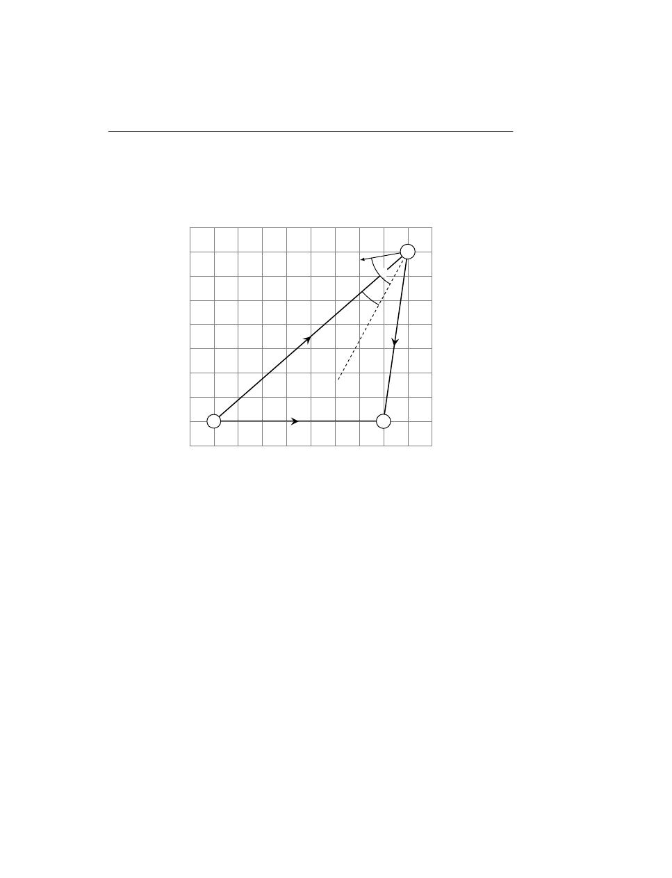
30
1. Introduction
of these items may be categorized as ground-based, airborne or marine and can be moving or be
stationary. The angle between vectors defined by the illumination path and the echo path (positive
angle, less than 180
◦
) is called a bistatic angle and is denoted with β. It is also sometimes called
the cut angle or the scattering angle. Another crucial angle is the aspect angle denoted by δ and it
defines the target’s movement at speed v with respect to the bistatic bisector.
Direct path
Baseline L = d
TR
Echo
path
d
AR
Illumination
path
d
T
A
v
δ
β/2
T
R
A
Figure 1.2: Bistatic triangle with accompanied features and variables.
The distance between the transmitter T and the receiver R is not explicitly given in the definition
of bistatic radar. However, in Skolnik (2003) the author quantifies the separation as one of “a
considerable distance” or “comparable with the target distance” or “the echo signal does not travel
over the same path as the transmitted signal”.
1.5.1
Passive bistatic radar
One of the forms of Bistatic Radar is the Passive Bistatic Radar. Passive Bistatic Radar is also
known as bistatic hitchhiker or parasitic radar and it uses illuminators of opportunity as transmitters
to track an object.
In general the concept of the PBR can be specified as:
• PBR is a subtype of BR (all bistatic analysis such as geometry, doppler, RCS apply),
• PBR is a BR that does not emit any Radio Frequency (RF) of its own to track targets,
• it utilizes the existing RF energy in the atmosphere,
• as sources of RF energy we can use broadcast Frequency Modulation (FM) stations, GPS,
cellular telephones and commercial television,

1.5 Bistatic radar
31
Merits
Disadvantages
no demand for frequency allocation
no direct control over emitted signal
relatively low cost
complicated geometry with respect to
monostatic radar
covert receiver location, no possibility of
jamming
technology is outdated
immune
to
Anti-Radiation
Missiles
(ARM)
possibility to detect stealth objects
good low level coverage
large number of transmitters
complements existing system
Table 1.1: Merits and disadvantages of PBR usage.
• Hitchhiker or parasitic radar are used in a case when another radar transmitter is used, such
as signal from monostatic radar,
• when the transmitter of opportunity is from a non-radar transmission, such as broadcast com-
munications, then terms such as passive radar, passive coherent location or passive bistatic
radar are used.
The common use of PBR is to use RF energy such as commercial FM broadcast as a transmitter T
which is scattered by an aircraft A. Reception of the scattered signal is conducted with an antenna
and compared with the reference signal (direct path signal) from a second receiving antenna. Then
by using Digital Signal Processing (DSP) techniques, target-related parameters such as range, range-
rate, Angle of Arrival (AoA) and other can be estimated.
An alternative method is the Doppler-only technique which does not use a second receiving antenna,
but rather a system of bistatic radars working in unison. The received signal is analyzed by putting
great importance on Doppler shift information. The information acquired by the receiving parties
involved is then combined in order to detect/track targets.
Merits and disadvantages of using a PBR configuration are presented in Table 1.1.
Examples of such transmitters are analog radio/tv transmitters, cellular phone base stations and
Digital Audio Broadcast (DAB) that have been presented in Griffiths and Baker (2005); Malanowski
et al. (2014) or Global Navigation Satellite System (GNSS) in Clemente and Soraghan (2014);
Suberviola et al. (2012).
1.5.2
History in brief
First experiments on Bistatic Radar have been conducted simultaneously in United Kingdom, The
United States, France, the Soviet Union, Japan, Germany and Italy in the late 1930s, before the
Second World War. Some of the experiments were deployed as forward scatter fences (along country
32
1. Introduction
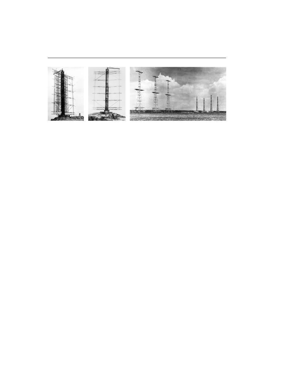
Figure 1.3: A Klein Heidelberg in Tausendfüssler near Cherbourg (left) and at Biber (middle).
Towers of British Chain Home (right).
borders) or as a bistatic hitchhiker as an aircraft detection systems. These radars were known as
Continuous Wave detectors and served to detect an object as it crossed the baseline by estimating
the frequency of the Doppler shift caused by an airborne object with respect to the direct signal
path from transmitter T to a parasitic or dedicated receiver R. In 1930 an aircraft was accidently
spotted by L.A. Hyland while working on the directional properties of an aircraft antenna system at
32.8 MHz and being located 3.2 km from the aircraft. Two years later a team of Taylor, Young and
Hyland used bistatic radar to detect aircraft 80 km from the transmitter. In 1935 Britons Watson-
Watt and Arnold Wilkins conducted an experiment of aircraft detection in a forward-scatter fence
configuration which later on was developed into the Chain Home network (see Fig. 1.3) of radars
along the British coast. The network appeared to be effective during the Battle of Britain in 1940.
In Germany bistatic radar was developed during World War II under the name Klein Heidelberg, see
Fig. 1.3. It was using the British Chain Home radar as an illuminator of opportunity and was used
to detect approaching allied bombers when they were passing the English Channel.
The first wave of interest in BR ended in mid 1930s. The interest was revived in 1950s when the
development in monostatic radar theory, techniques and technology could be used also in a bistatic
configuration. During this time a couple of new theories were introduced including Bistatic Radar
Cross Section (BRCS) and bistatic clutter measurement. Development of semiactive homing mis-
siles and a second attempt at hitchhiking and forward-scatter fences took place. This time hitchhik-
ing was aimed at locating objects in space using atmospheric phenomena, such as lighting or radio
stars like the Sun, as transmitters. Multistatic radars were designed with the purpose of ballistic
missile detection in systems like the U.S. Plato, satellite detection and tracking fence Navsparus.
Only the last one was actually deployed.
The second resurgence of the BR subject is dated to 1970s. During these years several new systems
were introduced including Sanctuary, presented in Bailey et al. (1977), Bistatic Alerting and Cueing
(BAC) in Thompson (1989), Aircraft Security Radar (ASR) and Multistatic Measurement System
(MMS) in Willis (2005).
The main objective of the Sanctuary project was to generate a clutter-free display for air defense
operations with a transmitter onboard of an aircraft and ground-based coherent receiver. Success-
ful flight tests were performed during which jet attack aircraft was detected at range greater than
100 km.
The ASR on the other hand had a purpose of detecting intruders approaching an aircraft. The

1.5 Bistatic radar
33
configuration of this fence-like system was based on five bistatic pulse-Doppler radars operating
at 5.8 GHz and arranged around the aircraft to be protected. Each of the five points consisted of
a collocated transmitter and receiver, so besides the bistatic fence the system was supported by
monostatic radar information.
1.5.3
Nonmilitary applications
One of the most prominent nonmilitary application was to use an orbiting Continuous Wave trans-
mitter and earth-based receiver to construct a lunar map by sampling interference patterns between
direct and echoed signals. It has been employed during the moon flights of Lunar Orbiters 1 and 3,
Explorer 35 and Apollo 14 and 15. Mapping of Venus was conducted by USSR with Venera 9 and
10 satellites. The thickness of the Saturn’s rings was estimated using microwaves traveling from
Voyager 1 through the rings towards the Earth, as described in Zebker and Tyler (1984).
Bistatic radar was also used to determine the frequency and direction of travel of waves on the
surface of the sea with two Loran-A transmitters located on Hawaiian Islands and the receiver on
board a ship, Peterson et al. (1970).

34
1. Introduction

C
HAPTER
II
Used techniques
In this chapter techniques used in Chapters 4,5,6 are presented. We assume that the signal that is
taken under consideration during the presentation of the techniques is denoted by s and it is a one
dimensional sequence dependent on time t.
2.1
Discrete Fourier Transform
In Cohen (1989) the author reviews a number of methods of joint time-frequency distributions and
how the spectral content changes over time. Among many distributions we can list a few of the most
popularly used:
• Wigner-Ville distribution and its smoothed version,
• Spectrogram,
• Rihaczek-Margenau-Hill distribution and Windowed-Rihaczek-Margenau-Hill distribution,
• Choi-Williams distribution,
• B distribution, Modified B distribution and Extended Modified-B Distributions
• Compact Support Kernel based Distributions and Extended Compact Support Kernel based
Distributions,
• Short Time Fourier Transform (STFT),
• Born-Jordan distribution,
• Zhao-Atlas-Marks distribution,
• Cross Wigner-Ville distribution,
• Polynomial Wigner-Ville distribution (order 6 kernel and order 4 kernel),
• Ambiguity Function
35
36
2. Used techniques
In this work STFT is used to represent a signal in the time-frequency domain.
When calculating the Fourier Transform (FT) of some given function, it might happen that it is
defined in terms of a continuous independent variable, like in the case of transform pairs. In the
case when function values are given as discrete values at regular time intervals, like with physical
measurements, the transformed function will also be available at discrete intervals. One may think
of a discrete function as a sort of approximation of an underlying function of a continuous variable.
To understand the Discrete Fourier Transform (DFT) one must understand the idea of periodicity.
A periodic function is a function the values of which are repeated at equal intervals of T seconds.
We can say then that the values are repeated with frequency
1
T
Hz.
Let us assume that the parameter τ represents a time with N consecutive integer (positive) values.
To illustrate the discretizing operation, let us take the sine function on interval [0,
3
2
π], see Fig. 2.1.
1
2
3
4
5
−1
0
1
t
h
ar
(t
)
5
10
15
−1
0
1
τ
f
ar
[τ
]
Figure 2.1: An example of the discretization of the sine function. Note the change in scale on
horizontal axes for continuous time t and discrete time τ .
The domain notation has changed from continuous time notation t to a discrete one τ , thus for the
function sine, values of h
ar
are only known at discrete time instances f
ar
[τ ]. We can summarize this
operation by formulae 2.1.
f
ar
[τ ] = h
ar
(t
0
+ τ T )
(2.1)
where T stands for the sampling interval and t
0
denotes time occurrence of the first sample. The
definition of DFT given in Bracewell (2000) states that f
ar
[τ ] possesses a discrete Fourier transform
F (v) expressed by
F (v) = N
−1
N −1
τ =0
f [τ ] e
−i2π(v/N )τ
(2.2)
It is important to stress that there are different frequency notations for the continuous case and the
discrete one. The frequency notation for FT is f , whereas for DFT it is v/N which can be interpreted
as quantity measured in cycles per sampling interval.
The DFT shares all the properties of FT. However the form of these properties may be different.
Using the functional operator F , which converts a function to its Fourier transform, we assume that

2.1 Discrete Fourier Transform
37
F [f
ar1
[τ ]] = F
ar1
(e
iτ ω
) and F [f
ar2
[τ ]] = F
ar2
(e
iτ ω
), where ω = 2πv/N , f
ar1
and f
ar2
are two
discrete signals (functions dependent on discrete time τ ).
• linearity
F [af
ar1
[τ ] + bf
ar2
[τ ]] = aF
ar1
e
iτ ω
+ bF
ar2
e
iτ ω
,
• time shifting
F [f
ar1
[τ − τ
0
]] = e
−iτ
0
ω
F
ar1
e
iτ ω
,
• time reversal
F [f
ar1
[−τ ]] = F
ar1
e
−iτ ω
,
• frequency shifting
F f
ar1
[τ ] e
iω
0
τ
= F
ar1
e
iτ (ω−ω
0
)
,
• differencing
F [f
ar1
[τ ] − f
ar1
[τ − 1]] = 1 − e
−iτ ω
F
ar1
e
iτ ω
,
• differentiation in frequency
F
−1
i
d
dω
F
ar1
e
iτ ω
= τ f
ar1
[τ ] ,
• convolution theorems
F [f
ar1
[τ ] ∗ f
ar2
[τ ]] = F
ar1
e
iτ ω
F
ar2
e
iτ ω
F [f
ar1
[τ ] f
ar2
[τ ]] = F
ar1
e
iτ ω
∗ F
ar2
e
iτ ω
,
• Parseval’s relation
∞
τ =−∞
|f
ar1
[τ ]|
2
=
1
2π
2π
0
F
ar1
e
iτ ω
2
dω
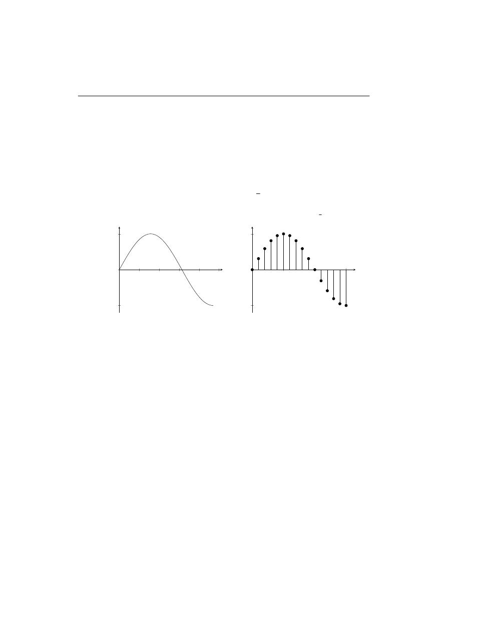
An example of DFT in a form of amplitude signal is presented in Fig. 2.2. Here as an input
signal the summation of two sine functions is taken, such as f
ar
[τ ] = 5 sin (2πτ f
1
+ π/4) +
2 sin (2πτ f
2
− π/2) + e, where f
1
= 45 Hz, f
2
= 110 Hz and e ∼ N (0, 1) denotes a source of noise
that follows the normal distribution. Sampling frequency is equal f
s
= 1 kHz which means that time
length of the sample presented in Fig. 2.2 is equal τ /f
s
= {1, ..., 500} /1000 = {0.001, ..., 0.5} s,
0.5 s.
The spectrum in Fig. 2.2 depicts the signal after the transformation. The peaks represent the main
periodic components of the signal under consideration. The first peak is located at 44.92 Hz, the sec-
ond one at 109.4 Hz. This inaccuracy in frequency determination compared to the original settings
is due to the length of the signal – the more samples of the signal the better the frequency estimation.
The reason the amplitudes on the spectrum are not exactly 5 and 2 (these are estimated as 5.04 and
1.74, respectively) is due to the noise e. The remedy for this is as in the case of frequency inaccuracy
is to increase the length of the considered signal.
38
2. Used techniques
0
100
200
300
400
500
−5
0
5
10
discrete time τ
f
ar
1
[τ
]
0
100
200
300
400
500
2
4
frequency Hz
|F
[f
ar
1
]|
Figure 2.2: Original discretized signal (left) and its single-sided amplitude spectrum (right)
2.2
Short Time Fourier Transform
The STFT is a significant tool of time-frequency representation in fields like radar (Rothwell et al.,
1998; Pan et al., 2013), sonar (Ferguson, 1996), music (Pielemeier et al., 1996), speech (Liu, 1993),
(instantaneous) Frequency Modulation (FM) demodulation (Kwok and Jones, 2000). Due to the
demand of quick execution time, an efficient instantaneous implementation of the STFT is essential.
The merits of STFT over other time-frequency distributions are presented in (Durak and Arikan,
2003).
In order to transform a signal f
ar
with STFT (Allen and Rabiner, 1977), also known as short-time
spectrum (Hlawatsch and Boudreaux-Bartels, 1992), into matrix form (spectrogram image) with
time-frequency (t, ω), domain expressed in s and Hz, the following equation 2.3 must be used
S (t, ω) =
N −1
τ =0
f
ar
[τ ] w [τ − tG] e
−iωτ
(2.3)
where f
ar
(τ ) is an input signal at time τ , w is a length L window function, S(t, ω) is the Discrete
Fourier Transform of windowed data centered about time tG and G denotes a hop size (in samples)
between successive DFTs. Further we will refer to S, S(t, ω) as the spectrogram resulting from the
STFT operation.
The procedure of applying STFT to the signal might be outlined as follows:
• Split the signal into blocks of equal length L,
• The blocks overlap each other by some factor 100 % > 1 −
G
L
% ≥ 0 %,
• Each consecutive block is windowed. The windowing operation is a multiplication of the
block with a smooth function with tails that are nearly zero.
In Oppenheim and Schafer (2009), the authors list window functions typically used for smoothing:
2.2 Short Time Fourier Transform
39
• Rectangular
w [n] = 1, 0 ≤ n ≤ L,
• Hann
w [n] = 0.5 − 0.5 cos
2πn
L
, 0 ≤ n ≤ L,
• Hamming
w [n] = 0.54 − 0.46 cos
2πn
L
, 0 ≤ n ≤ L,
• Blackman
w [n] = 0.42 − 0.5 cos
2πn
L
+ 0.08 cos
4πn
L
, 0 ≤ n ≤ L,
• Kaiser
w [n] =
J
0
η 1 −
2n
L
− 1
2
1
2
J
0
(η)
, 0 ≤ n ≤ L.
with J
n
, n = 0 the zeroth-order modified Bessel function of the first kind. Rectangular for
η = 0, gaussian for η → ∞.
Shapes of the listed window functions are presented in Fig. 2.3.
0
L
2
L
0
0.5
1
n
w
[n
]
Rectangular
Hann
Hamming
Blackman
0
L
2
L
0
0.5
1
n
w
[n
]
η = 1
η = 2
η = 5
η = 10
η = 20
η = 50
Figure 2.3: Window functions. Rectangular, Hann, Hamming, Blackman (left). Kaiser with param-
eter η = {1, 2, 5, 10, 20, 50} (right).
One of the significant properties of STFT is its ability to represent time-frequency content of signals
that is free of cross terms as presented in Durak and Arikan (2003). The existence of cross-terms
however can be observed when using other transforms such as Wigner Distribution (WD). Here the
cross-term existence is due to the auto-correlation function inherent in its formulation. Cross-term
elimination is an important quality for distinguishing real components from artifacts which is crucial
for the case presented in this work, therefore further analyzes here are based on STFT application.
The other important feature of STFT is its computational simplicity. In general the properties of
STFT with respect to other time-frequency analysis transforms can be summarized as

40
2. Used techniques
• the clarity of representation is of low quality,
• the fixed resolution issue. The width of a window is a trade-off between time and frequency
resolution. Longer window (narrowband) lead to higher frequency resolution but decreases
time resolution which can be observed as smudges (smoothing) in time direction. The short
window (wideband) determines high time resolution and low resolution in frequency, which
is also undesired,
• cross-term free transform,
• low computational complexity.
By multiplying one of the aforementioned window functions with the window of the signal we
attenuate the middle part and suppress the tails of the windowed signal which characterizes STFT
as a local spectrum of the signal around the analysis window.
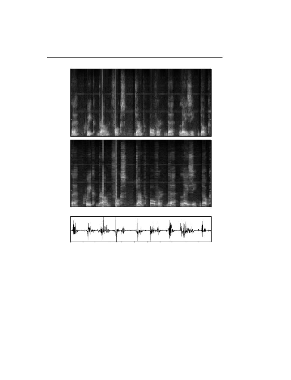
An example of the application of Short Time Fourier Transform is depicted in Fig. 2.4.
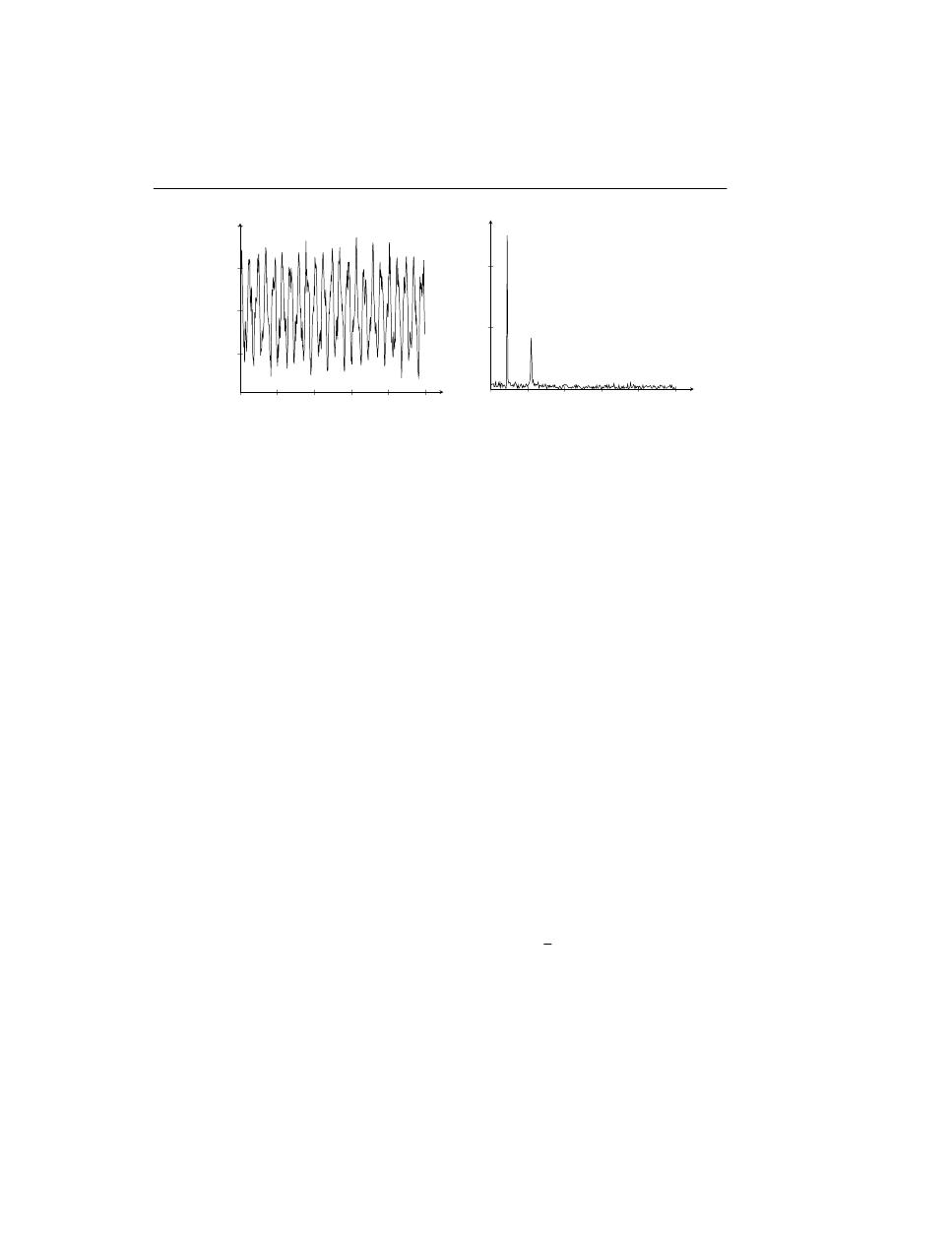
Here we consider recorded speech of the sentence The quick brown fox jumped over the lazy dog.
The example ought to show how the one dimensional signal (bottom) can be represented in a more
informative and intuitive way which is a two dimensional time-frequency domain (center and top).
The top two first images are presented to visualize a difference between different window sizes L.
The first image represents STFT with window width L = 1 ms which can be interpreted as a good
trade-off between the resolutions of the signal of 44 100 Hz sampling frequency f
s
. The purpose
of the second image is to show how the undesirable smoothing factor, lack of sharpness in time
direction, for STFT come into play for window width L = 10 ms.
2.3
Cell Averaging Constant False Alarm Rate
As mentioned in 2.2 a matrix of spectrogram data is denoted by S
[n×m]
and an amplitude of each cell
of this matrix by S (t (p) , ω (j)), where t (p) , p ∈ [1, n] denotes a time for the cell being measured,
and ω (j) , j ∈ [1, m] the frequency that corresponds to the cell. n and m are sizes in time and
frequency domains, respectively, of the spectrogram.
Constant False Alarm Rate (CFAR) technique is well documented, and many variants of it have
been developed.
As an example of this technique we want to give a brief presentation of one of the aforementioned
models, namely the Cell Averaging – Constant False Alarm Rate (CA-CFAR).
Let us consider Fig. 2.5 in which there are three distinguished groups of cells: reference cells
(dotted), guard cells (crosshatch), and the Cell Under Test (CUT) (grid). To check if detection is
declared in the CUT we need to average over all the reference cells RC of length n
RC
and then after
multiplying it with the constant k
CF AR
compare with the amplitude of CUT, see (2.4).
S (t (k) , ω (p)) > k
CF AR
1
n
RC
j∈RC
S (t (k) , f (j))
(2.4)
where RC denotes a reference cell’s location in the frequency domain and is of length n
RC
, k
CF AR
stands for a scaling constant. If the inequality is satisfied then CUT is stored and denoted as
S (t (k) , ω (p
i
, t (k))) , p
i
∈ [1, m].
2.4 Vincenty’s Inverse Formulae
41
0
2
4
6
8
frequenc
y
kHz
0
2
4
6
8
frequenc
y
kHz
0
0.5
1
1.5
2
2.5
3
3.5
4
4.5
5
time s
The
quick
brown
fox
jumped
over
the
lazy
dog
Figure 2.4: Recording of the sentence The quick brown fox jumped over the lazy dog with sampling
frequency f
s
= 44 100 Hz (bottom); spectrum representation with Hamming window of length
L = 1 ms and overlapping ratio of 50 % (top); the spectrum with L = 10 ms, 50 % (center).
2.4
Vincenty’s Inverse Formulae
Assuming that flight trajectories are presented in spherical coordinates the following formulae is
applied in order to calculate the geodesics.
In Vincenty (1975), the author presents a new method for deriving the shortest distance between
two arbitrary locations (length of geodesics) on the Earth. The method features a relatively high

42
2. Used techniques
t (p − 1)
t (p)
t (p + 1)
ω
(1)
ω
(p
i
)
ω
(m
)
Reference cells
Guard cells
CUT
Figure 2.5: Cell averaging constant false alarm rate scheme.
precision (down to 0.6 mm accuracy) and low time consumption, so it is used often in applications.
The compactness of the formulae is due to nested equations to compute elliptic terms. From two
techniques presented by Vincenty, the direct and the inverse, we need to use Vincenty’s Inverse
Formulae (VIF), which is an iterative approach and is sketched in the following blocks:
ψ = L
V
(2.5)
sin
2
ξ = (cos U
2
sin ψ)
2
+ (cos U
1
sin U
2
− sin U
1
cos U
2
cos ψ)
2
(2.6)
cos ξ = sin U
1
sin U
2
+ cos U
1
cos U
2
cos ψ
(2.7)
tan ξ =
sin ξ
cos ξ
(2.8)
sin α = cos U
1
cos U
2
sin ψ
sin ξ
(2.9)
cos 2ξ
m
= cos ξ − 2 sin U
1
sin U
2
cos
2
α
(2.10)
u
2
=
cos
2
α (a
2
− b
2
)
b
2
(2.11)
parameter ψ is derived from equations 2.12 and 2.13
C =
f
E
16
cos
2
α 4 + f
E
4 − 3 cos
3
α
(2.12)
ψ = L
V
+ (1 − C) f
E
sin α ξ + C sin ξ cos 2ξ
m
+ C cos ξ −1 + 2 cos
2
2ξ
m
(2.13)
The block of equations starting from equation 2.6 is being derived until the change in parameter ψ
is negligible (change of about 10
−12
). After that we evaluate the following
d
TR
= bA (ξ − ∆ξ)
(2.14)

2.4 Vincenty’s Inverse Formulae
43
T
α
1
d
TR
M
1
R α
2
N
ξ
m
ξ
1
ξ
E
M
2
Q
α
Z
Figure 2.6: Sphere with parameters used in Vincenty’s inverse formulae
where ∆ξ can be calculated from equations 2.15, 2.16 and 2.17
A = 1 +
u
2
16384
4096 + u
2
−768 + u
2
320 − 175u
2
(2.15)
B =
u
2
1024
256 + u
2
−128 + u
2
74 − 47u
2
(2.16)
∆ξ = B sin ξ cos 2ξ
m
+
1
4
B cos ξ −1 + 2 cos
2
2ξ
m
+
−
1
6
B cos 2ξ
m
−3 + 4 sin
2
ξ
−3 + 4 cos
2
2ξ
m
(2.17)
The azimuths may be estimated from equations 2.18 and 2.19
tan α
1
=
cos U
2
sin ψ
cos U
1
sin U
2
− sin U
1
cos U
2
cos ψ
(2.18)
tan α
2
=
cos U
1
sin ψ
− sin U
1
cos U
2
+ cos U
1
sin U
2
cos ψ
(2.19)
(2.20)
Notation for the Vincenty formulae.

44
2. Used techniques
a, b
major and minor semiaxes of the ellipsoid, a = 6 378 137 m, b =
6 356 752.314 245 m
f
E
=
a−b
a
flattening, f
E
= 1/298.257223563
L
V
difference in longitude
d
TR
length of the geodesic between T and R
α
1
, α
2
azimuths of the geodesic, clockwise from north (forward az-
imuths). α
1
is produced in the direction from T to R. α
2
is pro-
duced in the direction from R to Z
α
azimuth of the geodesic at the equator
U
1,2
reduced latitude, defined as tan U
1,2
= (1 − f ) tan ψ
ψ
difference in longitude on an auxiliary sphere
ξ
angular distance on the auxiliary sphere from T to R
ξ
1
angular distance on the sphere from the equator to T
ξ
m
angular distance on the sphere from the equator to the midpoint
of the line M
1
Values for a, b and f
E
are taken from World Geodetic System 84 (WGS84).
2.5
Canny Operator
Canny operator also known as Canny edge detector (Russell and Norvig, 1995) is a standard al-
gorithm used for detecting edges in images, in this case it is used to estimate edges within the
spectrogram S (t, ω). To detect an edge within the spectrogram S at any orientation, the spectro-
gram must be convolved with two filters f
V
= G
σ
(x) G
σ
(y) and f
H
= G
σ
(y) G
σ
(x), where f
V
and f
H
are vertical and horizontal filters, respectively, and G
σ
(x) is a Gaussian function expressed
in equation 2.21
G
σ
(x) =
1
√
2πσ
e
−x2
2σ2
(2.21)
where σ denotes standard deviation. The differentiated form of the Gaussian function is derived in
equation 2.22
G
σ
(x) =
−x
√
2πσ
3
e
−x2
2σ2
(2.22)
The procedure used in Canny edge detector can be specified as follows
i. Calculate convolution of the spectrogram S with filters f
V
(x, y) and f
H
(x, y). The resulting
images are denoted with W
V
(x, y) and W
H
(x, y). Let us also define W (x, y) = W
2
H
(x, y) +
W
2
V
(x, y)

2.6 Hough Transform
45
ii. Calculate the absolute value of W (x, y)
iii. Search for the values in |W | (x, y) that are higher than some specified threshold T r.
The marked edge pixels are then linked together to form edge curves. This can be achieved by
making the assumption that any neighboring pixels (cells of matrix W ), that were found after the
threshold operation and that keep the orientation consistent, must belong to the same edge curve.
In Canny (1986) the author summarizes the performance criteria to include the following:
• Performance in detection ensures a low probability level of misdetection of real edge points,
and low probability level of detecting non-edge points. Maximizing Signal to Noise Ratio
(SNR), both probabilities can achieve significantly lower values.
• Detected edge points (cells) should be located as close as possible to the real edge’s center.
• Multiple detections of a single point must be avoided. The first criterion ensures that this
condition is filled by rejecting points that are considered false.
A one-dimensional example of applying the Canny operator is presented in Fig. 2.7. The convo-
lution of the signal presented in (i) is shown in c), the first derivative of the Gaussian function
presented in equation 2.22 is shown in b). The maximum of the absolute value of the convolved
function represents the edge point, here peaking at around 150.
2.6
Hough Transform
The Hough Transform (HT) is a global processing method for boundary detection. The features that
may be extracted with use of HT are circles, lines, ellipses and two-dimensional shape identification
in general. There are many different versions of this technique, some of them aiming at reducing
algorithm’s time consumption and some at decreasing its memory usage like the one presented in
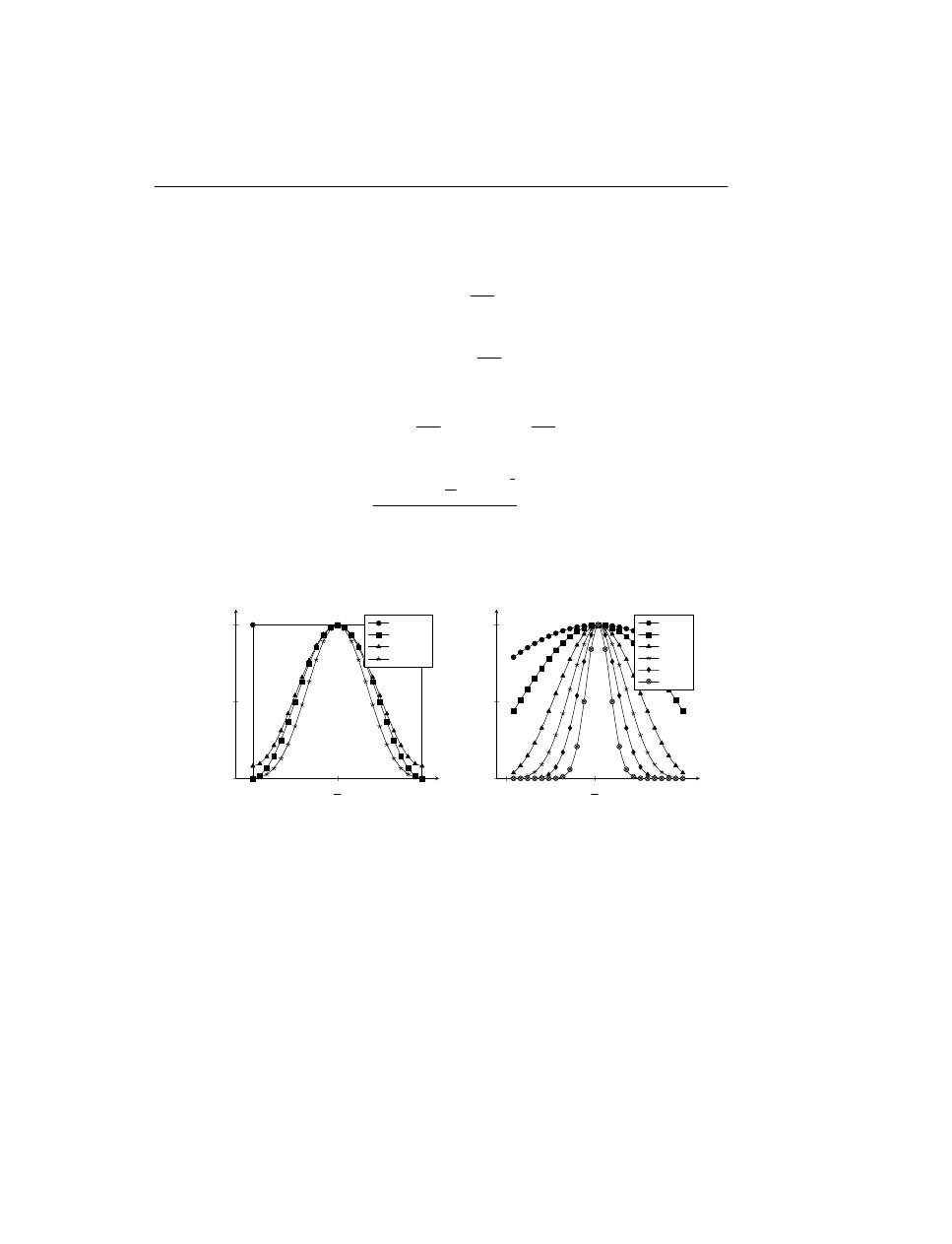
Chutatape and Guo (1999).
Firstly a binary edge image is estimated, with the use of the Canny operator f.e., after which each
edge point is transformed to a parameterized curve. The next step is to accumulate the accumulator
array which is usually implemented as an array of accumulator space. Each image pixel (cell of
matrix W ) gives one score to the cells lying on its transformed curve. The last step estimates the
local maxima. Cells with the local maximum of scores have coordinates of parameter representing
a curve (line) segment in the image space (matrix W ).
The kernel of the standard version of HT can be outlined as follows:
i. form the set W of all edge points in a binary image,
ii. transform each point of the set W into a parameterized curve of the parameter space,
iii. accumulate the accumulator space under each parametric curve,
iv. find accumulator cells that contain local maxima corresponding to image space curve param-
eters.
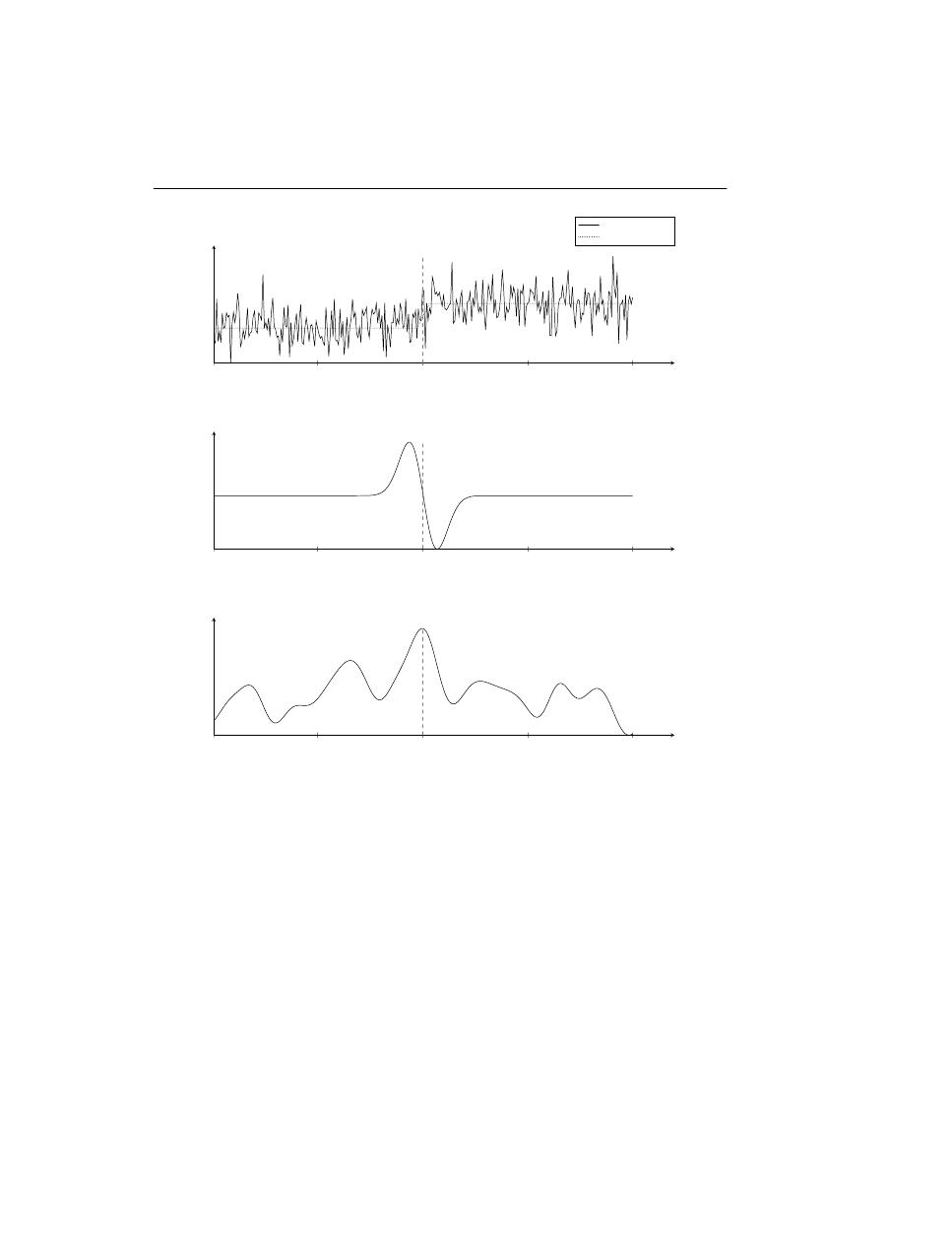
46
2. Used techniques
1
75
150
225
300
Function
Step function
Distorted step function
1
75
150
225
300
Derivative of Gaussian function G
σ
1
75
150
225
300
Convolution of the function
Figure 2.7: Canny operator applied to 1-D distorted step function.
In the following example the image is transformed to parametric representation which is presented
in equation 2.23.
ρ = x cos θ + y sin θ
(2.23)
where ρ is the distance from the origin to the line along vector perpendicular to the line, whereas
θ denotes the angle the normal line makes with the x-axis (the perpendicular projection from the
origin to the line measured in degrees clockwise from the positive half of the x-axis).
In Fig. 2.8 an application of HT to two straight lines is presented. The two lines were drawn with a
marker on a white piece of paper. As we can see the effect of the transformation presented in bottom
image drags our attention to two points marked here with 1 and 2, where the level of brightness is
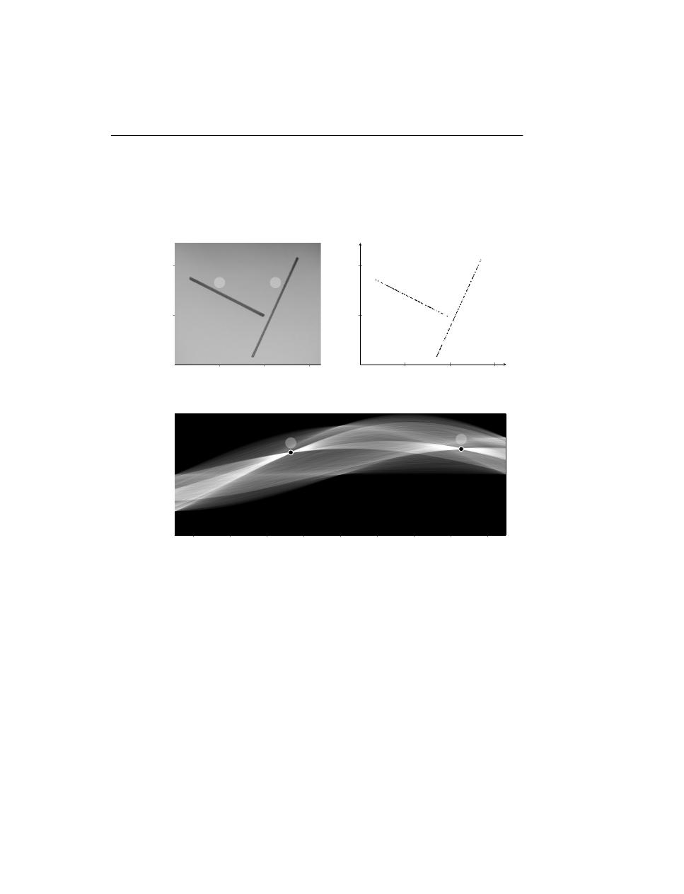
2.7 Bistatic radar equation
47
the highest which means it represents a high accumulation level. These points are a parametric
representation of the lines. The next step is to identify those local maxima from image space curve
parameters. Then the identified points are used for searching for line segments within the image
presented in top left. The result of this procedure is depicted in c).
1,000
2,000
3,000
1,000
2,000
1
2
a) Original image
1,000
2,000
3,000
1,000
2,000
c) Extracted features
−80
−60
−40
−20
0
20
40
60
80
−4,000
−2,000
0
2,000
4,000
1
2
θ
ρ
b) HT of the image
Figure 2.8: Hough Transform applied to an image. a) the image with two lines 1 and 2; b) HT of
the image in parameterized space (θ, ρ) with local maxima denoted as 1 and 2 corresponding to the
lines; c) extracted lines.
2.7
Bistatic radar equation
This section is presented assuming that in both cases of monostatic and bistatic radar the radar
waveform (transmitted signal) is in a form of repetitive series of rectangular pulses. Moreover its
purpose is to familiarize the reader with the concept of Bistatic Radar Cross Section (BRCS) which
is defined by the Bistatic Radar Equation (BRE).
Following the definition described in Skolnik (2008) and in Willis and Griffiths (2008) the equation

48
2. Used techniques
is expressed in (2.24) as
(d
TA
d
AR
)
max
=
P
av
T G
T
G
R
λ
2
σ
B
F
2
TA
F
2
AR
(4π)
3
kT
0
F
n
(E/N
0
) L
T
L
R
1
2
(2.24)
where
d
TA
transmitter to aircraft distance
[m]
d
AR
aircraft to receiver distance
[m]
P
av
transmitted average power
[J s
−1
]
T
signal observation time
[s]
G
T
transmitting antenna power gain
[1]
G
R
receiving antenna power gain
[1]
λ
wavelength
[m]
σ
B
BRCS parameter
[m
2
]
F
TA
pattern propagation factor for transmitter to aircraft path
[1]
F
AR
pattern propagation factor for aircraft to receiver path
[1]
k
Boltzmann’s constant
1.38 × 10
−23
[J K
−1
]
T
0
standard temperature
290
[K]
F
n
receiver noise figure
[1]
E/N
0
received energy to receiver noise spectral density required for
detection
[1]
L
T
transmitter system losses (>1)
[1]
L
R
receiver system losses (>1)
[1]
Comparison of the bistatic range equation with that of monostatic configuration (2.24) shows that the
form of the equation is similar. The definite difference is the replacement of d
2
T(R)A
with d
TA
d
AR
,
where d
T(R)A
denotes monostatic transmitter(receiver) to the aircraft distance. This replacement
causes fundamental changes to the operational system of Bistatic Radar (BR) compared to the
monostatic. One of these changes is that the region where the bistatic radar can operate is now
defined by ovals of Cassini, rather than a circle – as in the case of monostatic radar.
Non-collinearity of bistatic constant range sum, defined by d
TA
+ d
AR
, with bistatic constant de-
tection contours (ovals of Cassini) is another significant difference between monostatic and bistatic
configurations – in the case of monostatic radar these two contours, which are the circles, over-
lap each other. This causes aircraft’s E/N
0
parameter to change with respect to its location on a
constant range sum contour - in contrast to the constant value of E/N
0
for monostatic radar case.
The next difference is a varying width of bistatic range cell with respect to the target’s location on a
constant range sum contour (ellipse) – against a constant width for monostatic.
The fourth difference is given in a form of pattern propagation factors F
TA
and F
AR
which in the
case of monostatic radar are usually equal, whereas for the bistatic radar they almost always differ.
These four differences are given so as to understand the operational phenomena of bistatic radar
based on the easy-to-grasp monostatic radar operation. Therefore, for reference purposes, the mono-
static equation is presented in (2.25). Note that in the case of monostatic radar, usually both trans-

2.8 Bistatic Radar Cross Section
49
mission and reception are managed with the same antenna antenna.
d
2
T(R)A
=
P
av
GA
e
σ
M
E
i
(n) F
4
(4π)
2
kT
0
F
n
f
p
(S/N )
1
L
s
1
2
(2.25)
where
d
T(R)A
maximum radar range
[m]
G
TR
antenna gain
[1]
A
e
effective area of antenna
[m
2
]
σ
M
monostatic radar cross section of the aircraft
[m
2
]
n
pl
number of pulses
[1]
E
i
(n)
efficiency in adding n
pl
pulses
[1]
F
4
accumulation of propagation effects
[1]
f
p
Pulse Repetition Frequency (PRF) parameter
[Hz]
(S/N )
1
signal to noise ratio with one pulse present
[1]
L
s
system losses
[1]
2.8
Bistatic Radar Cross Section
In Willis and Griffiths (2008) the authors give the following definition of the Bistatic Radar Cross
Section.
Definition 2.8.1 The Bistatic Radar Cross Section (BRCS), denoted by σ
B
, is a measure of the
energy scattered from the target (aircraft) in the direction of the receiver.
The bistatic radar cross section is a function of bistatic angle β and aspect angle δ and therefore is
more complex than the monostatic Radar Cross Section (RCS).
Considering complex targets we can distinguish three regions of interest for BRCS with respect to
bistatic angle. They are:
i. pseudomonostatic, 0
◦
to 5
◦
ii. bistatic, 5
◦
to 180
◦
iii. forward scatter, ∼180
◦
By the term complex targets we understand a target that is built of discrete scattering centers, such
as flat planes, corner reflectors, dihedral with corner not equal to 90
◦
, stationary phase regions.
The first – pseudomonostatic region for complex targets is greatly reduced with comparison to
smooth, perfectly conducting targets such as sphere, ogive, cone, for which the region can extend to
β = 100
◦
for a sphere. Therefore the BRCS of complex targets can be reduced to monostatic one,
measured on the bisector of the bistatic angle at a frequency reduced by a factor of cos (β/2), if
the bistatic angle does not exceed 5
◦
. This condition is stated as a variation of equivalence theorem
given in Kell (1965).

50
2. Used techniques
The second bistatic region starts at the bistatic angle for which the equivalence theorem fails to
determine the BRCS. As previously for complex targets under condition that target aspect angle
is fixed with respect to bistatic bisector, there are three sources of divergence, namely: the phase
between discrete echoing centers now changes; changes in level of energy radiated from discrete
echoing centers; and new echoing centers emerge and some centers disappear.
The third region of BRCS is called the forward scatter and relates to a bistatic angle approaching
180
◦
. Forward scatter configuration was introduced in 1.5.2. In Siegel et al. (1955) it is showed that
when bistatic angle β = 180
◦
the target’s BRCS is relatively small with comparison to the target’s
dimensions and equals σ
F
= 4πA
2
/λ
2
, where σ
F
denotes BRCS for forward scatter case. In this
case the target might be either smooth or a complex structures.
To obtain the BRCS of some object one must use a suitable technique. Several such techniques have
been developed and among them we can distinguish groups and subgroups as follows:
• Theoretical (Prediction techniques)
– Graphical Electromagnetic Computing (GRECO) (high frequency) (hua QIN and fa WANG,
2002),
– Method of Moments (MoM) (numerical method) (Bhattacharyya, 1991),
– Finite Intergration Technique (FIT) (numerical method) (Weiland, 1996),
– Fast Multipole Method (FMM) (numerical method) (Rokhlin, 1990; Coifman et al.,
1993; Song et al., 1997),
– Shooting and Bouncing Rays (SBR) (Baldauf et al., 1991),
– Closed form Physical Optics (CPO) (Jackson et al., 2010),
– Current Marching Technique (CMT) (Li et al., 2009),
– Finite Element Method (FEM) (Alfonzetti and Borzi, 2000)
• Practical (Measurement techniques)
– Pendulum method (Matsuo et al., 1970)
– outdoor measurements: scaled model, full scale object (Schetne and Mount, 1965; Lane
et al., 1999)
– indoor measurements, most often with use of anechoic chamber: scaled model (Gürel
et al., 2003), full scale object
Arriving at explicit formulae of BRCS for a given object is a very challenging task. Just a couple
discrete shapes have been solved for their explicit formulation. Among them there are sphere and
cylinder.
These shapes were used as an example of explicit formulae of BRCS profiles. The first one consid-
ered is a perfectly conducting sphere where emitter and transmitter are both polarized perpendicular
to the plane containing the direction of incidence and scattering. A perfectly conducting body in a
time-varying magnetic field supports surface currents that shield the magnetic field from the interior
of the body. The equations of BRCS for electric and magnetic fields (σ
e
and σ
e
for E-plane and
H-plane, respectively) for the sphere is derived in the following fashion.

2.8 Bistatic Radar Cross Section
51
σ
e
(β) =
λ
2
π
∞
n=1
(−1)
n
2n + 1
n (n + 1)
b
n
∂P
1
n
(cos β)
∂β
+ a
n
P
1
n
(cos β)
sin β
2
(2.26)
σ
h
(β) =
λ
2
π
∞
n=1
(−1)
n
2n + 1
n (n + 1)
b
n
P
1
n
(cos β)
sin β
+ a
n
∂P
1
n
(cos β)
∂β
2
(2.27)
where
a
n
=
(J
n
(k
w
r
s
))
H
(2)
n
(k
w
r
s
)
b
n
=
k
w
r
s
J
n−1
(k
w
r
s
) − nJ
n
(k
w
r
s
)
k
w
r
s
H
(2)
n−1
(k
w
r
s
) − nH
(2)
n
(k
w
r
s
)
H
(2)
n
(k
w
r
s
) = J
n
(k
w
r
s
) − jY
n
(k
w
r
s
)
(2.28)
J
n
, Y
n
and H
n
are nth-order Bessel functions (Carrier et al., 2005) of the first, second and third
kind, respectively, and P
1
n
denotes the associated Legendre function (Filloux et al., 1987) of order
n and degree 1, r
s
denotes the radius of the sphere and k
w
, k
w
=
2π
λ
is the wave number.
The results of applying (2.26) and (2.27) for different values of the sphere’s circumference k
w
r
s
is
presented in Fig. 2.9.
In the case of the cylinder the formulations of BRCS for vertical (electric field, E-plane) and hori-
zontal (magnetic field, H-plane) polarizations are given in (2.29) and (2.30), respectively.
σ
e
(β) =
2λ
π
∞
n=0
Ω
n
(−1)
n
J
n
(k
w
r
c
)
H
(2)
n
(k
w
r
c
)
cos nβ
2
(2.29)
σ
h
(β) =
2λ
π
∞
n=0
Ω
n
(−1)
n
J
n
(k
w
r
c
)
H
(2)
n
(k
w
r
c
)
cos nβ
2
(2.30)
where
Ω
n
=
1, n = 0
(2.31a)
2, n = 0,
(2.31b)
the primes denote derivatives with respect to the argument and H
n
is the Bessel function of the
third kind (Hankel function), r
c
denotes the radius. To derive the BRCS of a real cylinder the
obtained scattering width needs to be multiplied by the cylinder’s length. It is worth noting that the
BRCS solution is reliable if the wavelength is relatively small with comparison to dimensions of the
cylinder (it also applies to the sphere).
The resulting BRCS of the cylinder for various k
w
r
c
values are illustrated in Fig. 2.10.
In the case of the sphere and the cylinder, infinite sums were approximated by limiting these series
to 2k
w
r
s
and 2k
w
r
c
first elements for the sphere and the cylinder, respectively.
52
2. Used techniques
180
240
300
360
−30
−25
−20
β
◦
σ
(β
)
π
a
2
dB
k
w
r
s
= 3
H-plane
E-plane
180
240
300
360
−40
−30
−20
−10
β
◦
k
w
r
s
= 6
H-plane
E-plane
180
240
300
360
−40
−30
−20
−10
β
◦
σ
(β
)
π
a
2
dB
k
w
r
s
= 12
H-plane
E-plane
180
240
300
360
−40
−20
0
β
◦
k
w
r
s
= 21
H-plane
E-plane
Figure 2.9: Standarized BRCS as a function of bistatic angle of perfectly conducting sphere for
various values of k
w
r
s
.
2.8 Bistatic Radar Cross Section
53
180
240
300
360
−30
−20
−10
0
β
◦
σ
(β
)
π
a
2
dB
k
w
r
c
= 19
H-plane
E-plane
180
240
300
360
−40
−20
0
β
◦
k
w
r
c
= 38
H-plane
E-plane
180
240
300
360
−20
0
β
◦
σ
(β
)
π
a
2
dB
k
w
r
c
= 75
H-plane
E-plane
180
240
300
360
−20
0
β
◦
k
w
r
c
= 113
H-plane
E-plane
Figure 2.10: Standarized bistatic RCS as a function of bistatic angle of the cylinder for various
values of k
w
r
c
.

54
2. Used techniques

C
HAPTER
III
Experiments
This chapter introduces configuration of the Bistatic Radar (BR) system used for acquiring data for
further analyzes.
3.1
Passive bistatic radar scenario
The Passive Bistatic Radar (PBR) scenario used in this work was exploited with one transmitting
site T and one or two receiving sites R. The transmitter used as an illuminator of opportunity, not
synchronized with the receivers, is located in a suburb of Saint Petersburg, Russian Federation. The
receivers were located in the neighborhood of Joensuu, North Karelia, Finland.
Locations of both receiving parties R that were recording Radio Signal Data (RSD), J and M –
first letters of the names of the receivers’ operators, and the transmitting station T are depicted in
Fig. 3.2. One of the receiving sites was recording with two antennas, therefore the notation was
given J
1
and J
2
, for more details see 3.3. Further we will refer to J as a location rather than a
particular antenna, whereas M will refer to an antenna configuration and location.
Notable distances between receivers J, M – d
JM
, between the transmitter T and receivers J, M –
d
TJ
, d
TM
, are respectively d
J M
= 42.2 km, d
T J
= 301.8 km, d
T M
= 288.4 km.
3.2
Transmitter
The transmitter used for commencing the experiments was the 310 m TV tower built in 1962 with
mounted TV-broadcastning/Frequency Modulation (FM) transmission. The TV transmitter emits on
frequency f
t
, f
t
= 49.75 MHz. The Effective Radiated Power (ERP) of St. Peterburg’s TV station
used in this experiment was 149 kW. Until 1985 the tower stood at 316 meters. At that time the
antenna atop the tower was replaced with a more modern version that was six meters shorter.
The transmitting antenna is horizontally polarized and omnidirectional. The pattern of the antenna
is a doughnut so it radiates negligible amount of power in the air space directly above the tower
– the power is uniformly distributed in every direction on the horizontal plane. Because of the
omnidirectional pattern of the transmitter the directional density of radiated power is about 50 %
less than of the same ERP for a dipole (Szóstka, 2006). The omnidirectional antenna is used as a
55
56
3. Experiments
d
TJ
d
TM
d
JM
J
M
T
Figure 3.1: Geographical location of transmitter T and receivers J, M and distances between them.
comparison when arbitrary antenna’s directionality and energy gain is defined. The omnidirectional
pattern seems a natural approach for TV broadcasting – equal reception around the transmitter.
3.3
Receivers
The Radio Signal Data (RSD) was captured by the three receivers, J
1
, J
2
and M located near Joen-
suu, Finland. Receivers J
1
and J
2
correspond to the same geographical location but different antenna
configurations. The receiving antennas’ parameters were as follows:
• 4-element horizontal dipole array at about 14 m above ground, with dipole end dip directed to
Saint Petersburg transmitter to attenuate signal strength increase during carrier crossing, for
receiver J
1
,
• rotatable horizontal 4-element 50 MHz Yagi-Uda, gain about 5 dBd, height about 7 m above
ground, directive pattern typical to 5-element Yagis, for receiver J
2
, and
• long wire of 250 m, which is slightly directional to northeast and has almost similar back lobe
pattern to south west, for receiver M.
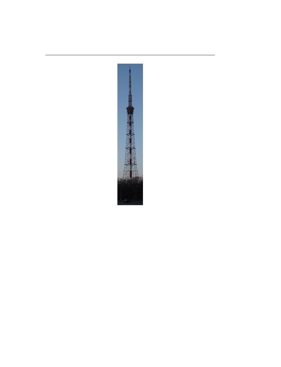
3.3 Receivers
57
Figure 3.2: Saint Petersburg TV tower.
The pictures of the Yagi and the Dipole antennas along with the associated schematics are presented
in Figures 3.4 and 3.5.
3.3.1
Dipole
Linear antennas are the oldest antennas and still the most popular antennas there are. The simplicity
combined with the performance of a half-dipole antenna creates a starting point for building more
complex structures such as: Yagi-Uda, the quad, the collinear, the loop. The simplest version of
the half-dipole consists only of a length of wire and it presents great possibilities to beginners, as
described in Carr and Hippisley (2011). The half-dipole belongs to a family of antennas named
Hertz
after Heinrich Hertz. His pioneering work includes discovering radio waves using a short
dipole in a 1887 experiment. The terms dipole, half dipole, half-wave dipole and half-wave doublet
are used interchangeably.
The half dipole is a balanced antenna meaning that it consists of a single conductor (wire, rod, tube,
etc.) of half-wave length λ/2. The fed is usually installed in the middle of the cut conductor in
which case the configuration is called a center-fed half dipole. The schematics of a center-fed half
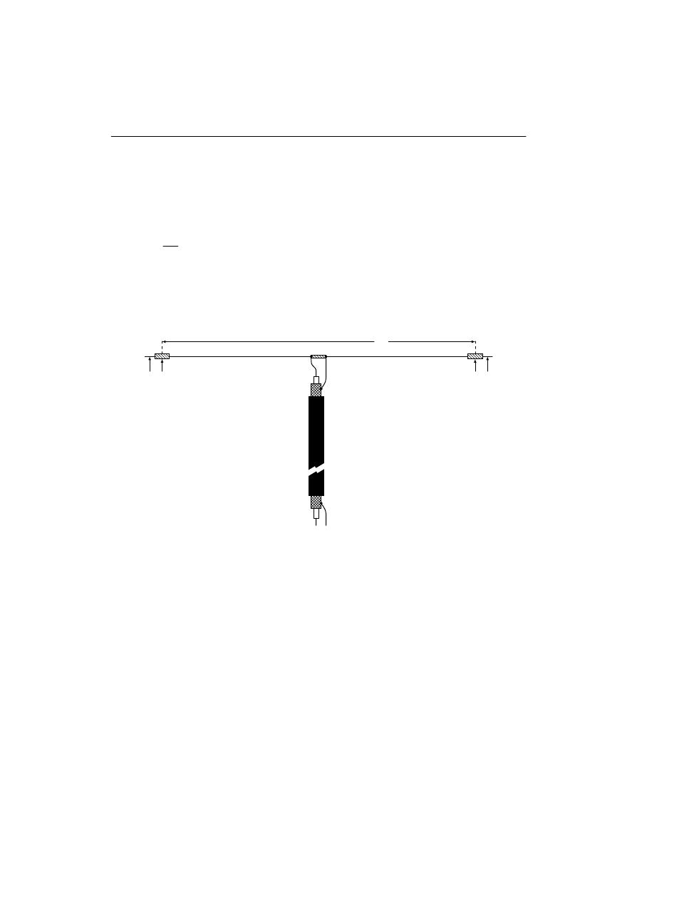
58
3. Experiments
dipole is presented in Fig. 3.3. Half dipole length is usually created to tune in to a certain frequency
in which case the length of the dipole is critical. The formulae which describes the relation between
the tuneable frequency, which is referred to as the transmitting frequency f
t
, and the length of the
dipole L
d
is presented in (3.1).
L
d
=
150
f
t
(3.1)
However the equation for the length of the conductor is only an approximation. Other parameters
that can affect the reception of transmitting frequency are antenna’s height above the ground, nearby
objects and length/diameter ratio of the conductor. To tune in to a transmitting frequency (to achieve
exact resonance), trimming or extending the conductor might be necessary.
75 Ω coaxial
I
c
s
I
I
R
R
L
Figure 3.3: Half dipole antenna. I - insulator, R - rope for stability purposes, c
s
- coaxial splitting
The construction of a 4-element half-wave dipole array is presented in Fig. 3.4. The Yagi used in this
study was located at about 14 m above ground and a gain of 4 to 5 dBd. It is almost omnidirectional
except for the dipole ends which are intentionally directed towards the chosen TV transmitter to
attenuate about 20 dBd of both the TV carrier and the high peak level of signal scattered from
aircraft during the moment of its carrier crossing.
From this point on J
1
will refer to a receiver with a dipole as the receiving array.
3.3.2
Yagi-Uda
As presented in Straw et al. (2007) the invention of the Yagi-Uda array is attributed to two Japanese
university professors Hidetsugu Yagi and Shintaro Uda from Tohoku University. The Yagi-Uda
array is commonly refered as a Yagi array.
The simplest configuration of a Yagi array consists of two parallel elements: the driven element and
a single parasitic element (Director or Reflector). This arrangement is called a 2-element Yagi. If the
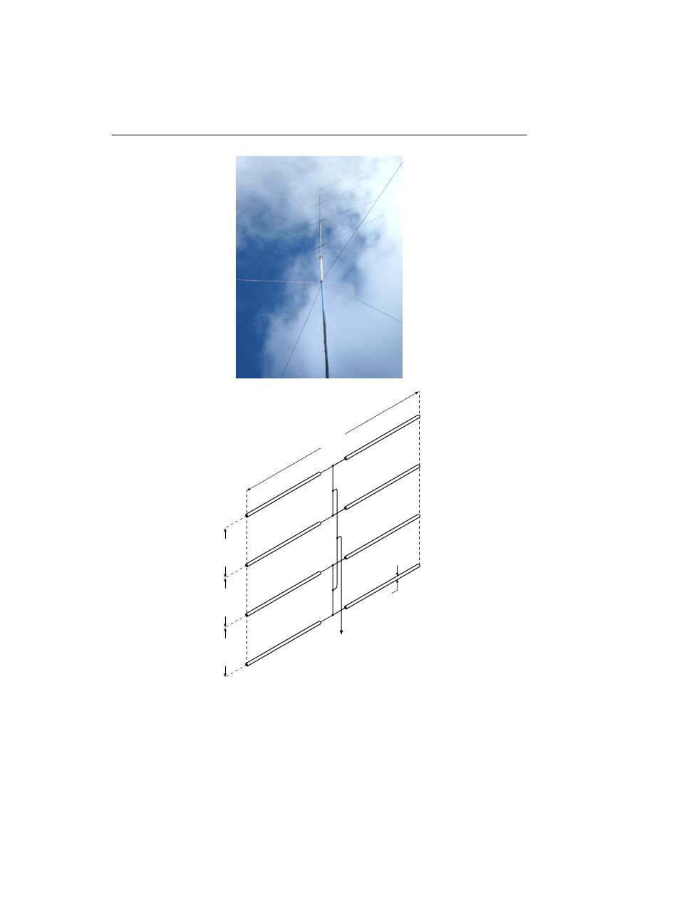
3.3 Receivers
59
c
s
c
s
c
s
c
s
c
d
c
d
c
d
2800
2000
2000
2000
3
50
Ω line
Figure 3.4: 4-element horizontal dipole array (top) together with its dimensional drawing. The
dimensions are given in mm. The c
s
points denote coaxial split, whereas the c
d
denotes coaxial
division.

60
3. Experiments
parasitic element is placed opposite to the maximum radiation direction, behind the driven element,
then it is called a reflector. Placing the parasitic element in front of the driven element gives it a
director
notation. A Yagi is engineered for Very High Frequency (VHF) and Ultra High Frequency
(UHF) frequencies and can include 30 or more director elements and a single driven element.
The gain and directional patterns of the array are a result of amplitudes and phases of currents
induced in every parasitic element, which on the other hand is given based on the spatial distance
between the driven element and parasitic elements and obviously the length and the diameter of the
elements. This implies that the operational idea of the Yagi array relies on mutual coupling of the
elements.
The following four parameters are relevant factors when it comes to characterizing a Yagi array:
i. Forward gain. Yagi free space gain (over an isotropic radiator in free space) ranges from
5 dBi for a basic 2-element configuration up to 20 dBi for a 31-element UHF design. The
main parameter that determines the gain is specified in terms of the length of the boom.
ii. Pattern. Gain is strongly determined by the antenna’s directivity pattern, in a particular by
the amount of energy accumulated in particular direction at the expense of energy radiated
in unwanted directions. A 3-element Yagi has a directional gain (main lobe of about 66
◦
for
3 dB loss compared to the peak gain at 0
◦
) of about 7.3 dBi over an isotropic antenna and
5.1 dBd over the half-dipole antenna. Separation of the frontal and rear originated signals is
yet another parameter determined by the directivity pattern. The antenna’s front-to-back ratio
measures the abilities of a Yagi to depress the unwanted rear (90
◦
to 270
◦
) interfering signal.
iii. Drive impedance/Standing Wave Ratio (SWR). The impedance of the driven element is af-
fected by the tuning of the driven element and the spacing and tuning of the parasitic elements.
In some cases inappropriate design of the Yagi can lead to a lack of stability between leading
performance parameters such as SWR, worst case Front-to-Rear ratio (F/R) and gain. In most
cases antennas purposed for high gain usually exhibit large changes of impedance levels with
relatively small changes in frequency. Therefore the SWR changes are wide which may lead
to unwanted changes in the feed cable.
iv. Mechanical strength.
All these parameters must be considered simultaneously to guarantee high receiving performance
and survivability of the array.
The Yagi array presented in Fig. 3.5, was design for reception of the VHF band, particularly for
signal reception of 49.75 MHz. The Yagi antenna will be referred further on as the J
2
.
3.4
Radio signal data
Radio Signal Data (RSD) was acquired using antennas described in 3.3.1 and 3.3.2. The receivers
J
1
, J
2
and M were tuned to record a spectrum of frequencies that includes the transmitter frequency
f
t
, (f
t
= 49.75 MHz) and accompanying Doppler curves. To obtain the spectrogram form of RSD,
Bracewell (2000), the Short Time Fourier Transform (STFT), presented in 2.2 was used with the
width of a symmetrically positioned Hann window L set to L =∼ 1 s, (8192 samples) and calcu-
lation time step G to G = 0.5 s. With these settings the spectrogram is categorized as overlapped
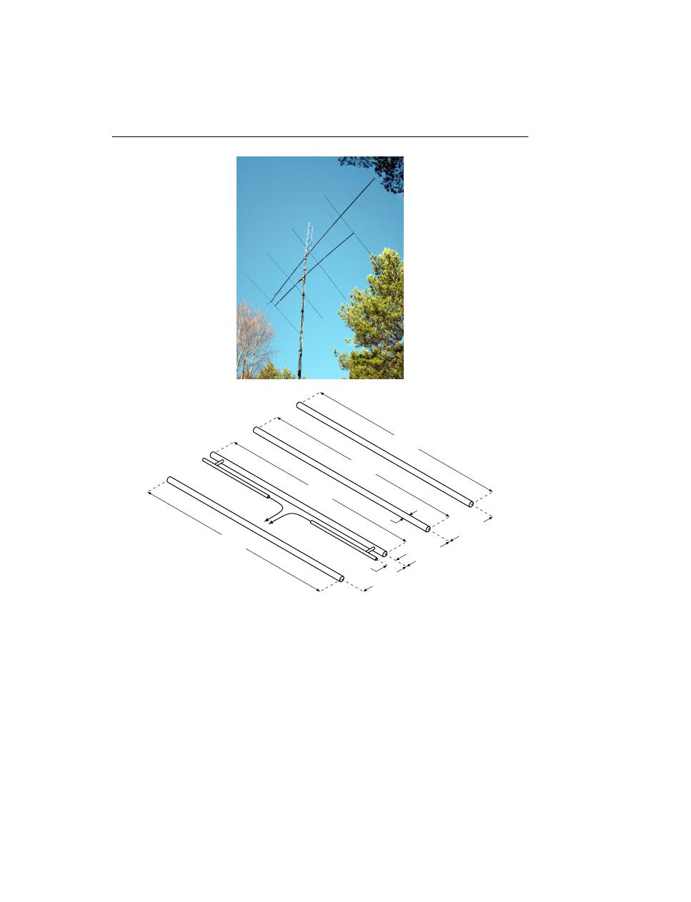
3.4 Radio signal data
61
2794
Radiator
50
Ω
line
2946
Reflector
2667
Director
2616
Director
1168
41
1168
1447
5
Figure 3.5: Dimensional drawing of the rotatable horizontal 4-element 49.75 MHz Yagi. The di-
mensions are given in mm.
with overlapping time of ∼ 0.5 s. This window specification ensures that information on the sig-
nal’s magnitude is not lost as stated by Izraelevitz (1985). Moreover, half-a-second time resolution
combined with 8192 samples per window provides a good time/frequency resolution for a Doppler
signature typically lasting some tens of minutes. By studying the Probability Density Function
(PDF) of the First Order Derivative of Doppler Shift (FODDS), described in Chapter 5, we can
deduce that a 0.5 s window will in most cases be sufficient to ensure steady and traceable transition
of Doppler signature in the time-frequency domain, discarding some extreme cases, such as aircraft
trajectories passing through the baseline or nearly parallel to it.

62
3. Experiments
3.5
Mode S data
In parallel, yet another type of data was collected from flightradar24.com website. This data is called
Flight Radar 24 (FR24). The web service provides information on aircrafts’ whereabouts based on
information sent and received using Automatic Dependent Surveillance - Broadcast (ADS-B) Mode
S IN and OUT protocols, respectively. The FR24 data consists of tracks of aircraft in proximity to
the transmitter T and the receivers J and M. The tracks on the other hand were built of the following
most relevant columns of data:
• latitude (latitudinal location of the aircraft), expressed in degrees (
◦
) with interval [−90, 90],
• longitude (longitudinal location of the aircraft), expressed in degrees (
◦
) with interval [0, 360],
• altitude (altitude of the aircraft above ground), expressed in meters (m),
• aircraft type designator International Civil Aviation Organization (ICAO), three or four char-
acter alphanumeric code associated with every aircraft type, defined by ICAO in ICAO (2012).
• wall-clock time of the sample being measured, expressed in seconds (s).
The extended list of data/message formats and control parameters for ADS-B Mode S specific ser-
vices are described in ICAO (2008). Each sample was collected in average every 5 s or 10 s, de-
pending on recording session settings.

C
HAPTER
IV
Long-distance passive multi-static aircraft tracking
In this chapter the multi-static Doppler radar concept based on long-distance Very High Frequency
(VHF) frequency recordings is presented and tested in a two receivers, one transmitter configu-
ration. The core of the method is a mathematical model of Doppler shift generation in a passive
configuration of many simultaneous transmitting radio stations and receivers that share the Doppler
shift information they have recorded. The tracking capabilities of such a multi-static configuration
are tested in an off-line experiment over a distance of 400 km. Aircraft position was recovered to an
apparent precision of 1500 m. The method also corrects for errors in time synchronization between
receivers.
4.1
Introduction
Air traffic safety is a global concern. Yet air safety radar systems are run to a large extent along
national boundaries. This has caused tragedies at times, like the disappearance of the Air France
flight 447 from Rio de Janeiro, Brazil, to Paris, France, over the Atlantic in 2009, where the avail-
ability of aircraft position over the Atlantic might have resulted in much faster detection of the
debris from the accident. There are examples where long-range aircraft monitoring might even have
prevented accidents, such as the disastrous mid air collisions in Ceritos (CA) 1986, Charkhi Dadri,
India 1996, Überlingen, Germany 2002 and Mato Grosso, Brasil 2006 might have been avoided, if
ground control were provided with correct and exact altitudes and positions of planes.
Part of this safety problem is caused by the inability of monostatic air surveillance radars to see be-
yond the range of their active radar beams. A multi-static radar solution using lower frequencies has
quite some potential in extending the view of air traffic radars to a more global scale. For instance,
Griffiths (2010) compares different radar systems and emphasizes in particular the advantages of
Multiple-Input and Multiple-Output (MIMO) radar systems over traditional monostatic ones. At
the moment, the development of transnational multi-static radar systems has been mostly left to
experimental setups. Some recent research devoted to the analysis and testing of multi-static sys-
tems can be found, for instance in Kuschel et al. (2008); Georgescu and Willett (2012) and Doughty
(2008); the issue of the target recognition in the micro–Doppler (µD) radar setup is considered, for
instance in Doughty (2008); Fogle and Rigling (2012).
In this chapter, a novel multi-static air surveillance approach is tested in a multi-static configuration.
It is a passive radar system based on commercial Very High Frequency (VHF) transmitters and
63

64
4. Long-distance passive multi-static aircraft tracking
individual radio amateurs. In particular, the DX listener community serves as the receivers. The
DX abbreviation comes from Distance Unknown (DX), and DX’ing is related to activity which is
listening to far away radio stations. The cross section of many pairs of radio stations and many
listeners can create a good global coverage for air traffic monitoring.
We test the viability of such a scenario in an off-line experiment where flight traffic is monitored
over a distance of some 400 km. Two radio amateurs are listening to a remote radio station and
recording the Doppler effect of flights crossing the line of transmission. From a combination of
their shifted Doppler measurements, the position of the aircraft is reconstructed off-line by means
of a mathematical model of the Doppler shift caused by an aircraft that first approaches and then
recedes from the line of transmission. The reconstruction of the flight path is compared to the
recordings obtained from the Automatic Dependent Surveillance - Broadcast (ADS-B) transponders
of the aircraft, as reported in the web service http://www.flightradar24.com.
The chapter is organized as follows. The second section explains relation between the paper and pre-
vious work on the subject. The third section presents the mathematical model developed. The fourth
section discusses the capture and processing of the data used in the experiment that is presented in
the fifth section. The chapter concludes with a discussion of the results obtained.
4.2
Previous research on bi and multi-static passive radar
Many authors have contributed methods that are related to the one presented here, but often in a
different context, such as real-time target tracking. In Howland (1999, 1995) the author used a bi-
static radar model with twin Yagi-Uda (3.3.2) antennas together with the Discrete Fourier Transform
(DFT) (2.1) and the difference between resulted phases of received signals in order to find estimates
for Doppler and bearings. Target echoes are identified with use of Cell Averaging – Constant False
Alarm Rate (CA-CFAR) (2.3) and then followed by Kalman Filter (KF) to associate individual
Doppler-Direction of Arrival (DoA) profiles. Finally the target’s coordinates and velocity are calcu-
lated with use of Genetic Algorithm (GA), Levenburg–Marquardt algorithm and Extended Kalman
Filter (EKF). The key to approximate target’s track is based on the use of two antennas horizontally
spaced, their phase interferometry is coupled with track estimation process which follows changes
in Doppler shift. Investigation of ground clutter by means of VHF airborne passive Bistatic Radar
(BR) was presented in Brown et al. (2012b). The paper discusses an application of Doppler Beam
Sharpening (DBS) to data collected from airborne receiver which resulted in producing graphical
representation of the area of interest. Successful experiment of detecting air targets by using air-
borne Passive Bistatic Radar (PBR) (1.5.1) with two antennas is presented in Brown et al. (2010).
However in Brown et al. (2012a) the airborne PBR experiment was repeated using a multi-static
radar architecture with two transmitters and compared with ADS-B Mode-S receiver records. The
resulted estimation of air target position was successful too. Ground based long range detection of
up to 700 km of bistatic range with use of Passive Radar Demosntrator (PaRaDe), Frequency Modu-
lation (FM) based PBR, was presented in Malanowski et al. (2012). The work discusses theoretical
limitations of aircraft detection range of PBR taking into account different factors such as Effective
Radiated Power (ERP) of the transmitter, receiver’s dynamic range, size of target, integration time.
Proposition of solving multi-static radar tracking system based solely on Doppler shift information
is demonstrated in Mixon (2012). The work presents strong mathematical basis for solving such a
system but also stresses that precision of measurement of Doppler shifts might prove to be crucial
for performance of presented algorithm.

4.3 Mathematical model
65
The approach presented here differs from previous study in it that it is genuinely multi-static, with an
arbitrary and possibly variable number of both transmitters - i.e. illuminators of opportunity – and
receivers. The architecture of the system is designed for passive, safety-focused monitoring of air-
traffic by volunteers using peer-to-peer exchange of flight information. Moreover, the detection of
aircraft from VHF Doppler-only signal is conducted with image processing of Doppler images and
mathematical optimization combined. In the current article we describe the algorithm to conduct
such multi-static passive flight trajectory detection and reconstruction and demonstrate its efficiency
with a real-life example, albeit an off-line one.
4.3
Mathematical model
This section presents the mathematical model to be applied to the Radio Signal Data (RSD) (3.4) in
order to estimate aircraft trajectories. The model uses spherical coordinates to calculate the distance
between two arbitrary points. All spherical distances are computed along geodesics and derived
from Vincenty’s Inverse Formulae (VIF) (see 2.4) which is accurate enough for the case presented
in this work. However, a technique presented in Karney (2013) can also be used. Hereafter J and M
refer to the receivers and I = {J, M} for notation simplification, T stands for the transmitter.
4.3.1
Preprocessing the data
The RSD consists of two time series of signals
s
I
(t)
I={J,M}
that have been recorded at two
different locations J and M.
Both sets have the same sample f
s
rate but a different recording start time t
0
I
and different recording
period T
r
I
.
To preprocess the RSD signals the following steps are taken.
First, the signals s
I
(t) are transformed with the Short Time Fourier Transform (STFT) (Allen and
Rabiner, 1977) into matrix form (spectrogram image) with time-frequency (t, ω) domain expressed
in s and Hz. Namely,
S
I
(t, ω) =
N −1
τ =0
s
I
[τ ] w
I
(τ − tG) e
−jωτ
(4.1)
where s
I
[τ ] is an input signal at time τ , w
I
(τ ) is a length L window function, S
I
(t, ω) is DFT of
windowed data centered about time tG and G denotes a hop size (in samples) between successive
DFTs. Hereafter the transformed signals are presented in a form of matrix denoted by S
I
(t, ω).
After operation presented in 4.1, the frequency domain of matrix S
I
(t, ω) is shifted as presented in
4.2
ω = ω −
ω
n
t=1
X
I
(t, ω)
n
= max
ω
n
t=1
X
I
(t, ω)
n
+ f
I
t
(4.2)

66
4. Long-distance passive multi-static aircraft tracking
where n is a size of matrix S
I
(t, ω) in time domain, ω denotes new domain of S
I
(t, ω) and f
t
I
is
the transmitting (carrier) frequency of the transmitted signal. In other words, the column of matrix
S
I
(t, ω) with the highest average amplitude is subjected to the shift f
I
t
. The range of ω remains the
same as the range of ω. This step is important as to ensure that the carrier signal is of the frequency
expressed in f
t
.
Next, the matrix S
I
(t, ω ) is reduced to S
I
(t, |ω − f
t
| < f
m
), where f
m
denotes the frequency
margin needed to enclose Doppler curves. For the sake of simplicity, we use S
I
(t, ω
∗
) instead of
S
I
(t, |ω − f
t
| < f
m
) in the text below.
4.3.2
The model
The theoretical model based mainly on data assimilation comprises the following steps.
• Heuristic approach to spectrograms analyzes based on Doppler history. Both spectrograms are
examined for possible pairs of Doppler curves. Namely, we look for any systematic difference
in time between appearances of Doppler curves on the two spectrograms. The time difference
and distance between receiving stations should coincide with the average cruise speed V
c
.
Once the pairs are identified, we focus on one of them and subject it to a further analysis.
• Time bounds. The region of the spectrograms S
I
(t, ω
∗
), where the Doppler curve is located,
is cut by time bounds s.t. t ∈
t
I
l
, t
I
u
. Let n
t
denote the size of matrix S
I
(t, ω
∗
) in the
time interval within the bounds t
I
l
, t
I
u
, where t
l
I
and t
u
I
denote lower and upper time limits
where the Doppler curve was found.
• Checking for swaying of the signal. Since the carrier frequency f
t
I
of the signal tends to sway
over time, we need to check its value for the previously defined region. This is done via the
formula in 4.3
f
I
t
=
ω
∗
n
t
t=1
S
I
(t, ω
∗
)
n
t
= max
ω
∗
n
t
t=1
X
I
(t
i
, ω
∗
)
m
t
(4.3)
Previously defined value of f
t
I
needs to be recalculated due to swaying phenomenon. It is de-
rived by calculating average value of spectrogram S
I
(t
i
, ω
∗
) along time domain and searching
for its maximum value. In this way we correct the value of f
t
. It is important to take this step
into account since further calculations rely on precisely defined value of f
t
.
• Edge detection. Next, the matrix S
I
(t, ω
∗
) is processed with the Canny edge operator (2.5)
with adjusted low and high thresholds. The Canny operator is superior to other edge detecting
methods for this case where the radio signal is fading in and out with time, see Canny (1986).
• Line search within spectrograms. The edge detected image (binary representation of matrix
S) is then used to find lines with the Hough Transform (HT). The choice of the HT parameters,
angle θ
I
and distance ρ
I
, depends on the shape of the Doppler curve. Finding lines within the
spectrograms is a key element as later they are used as reference lines for synthetic Doppler
fitting. We expect that found segments of lines mostly belong to Doppler curve. In this model,
we assume that Doppler curves emerge from straight-line-trajectories only. This assumption

4.3 Mathematical model
67
emerges from an idea that system is based on many BR connections thus the network of
bistatic lines is dense enough to ensure good approximation of trajectory even in the case of
aircraft’s change of azimuth. The result of the HT is a family of line segments described in
4.4
t =
1
sin θ
I
ρ
I
− ω
∗
cos θ
I
(4.4)
• The lines detected are used for the first estimation of the crossing time. The crossing time
is a time instant at which a family of lines crosses the carrier frequency. The crossing time
is estimated with the secant method and is denoted as t
x
I
further. This initial estimation of
the crossing time is not exact because it uses the HT with lines rather than with a model of
the radio signal itself that has a tangent function-like shape. However, it helps to eliminate
unwanted segments that are defined as the ones that satisfy the following condition
s.t.
t < t
I
x
∧ ω
∗
< f
I
t
(4.5a)
t > t
I
x
∧ ω
∗
> f
I
t
(4.5b)
The segments to be deleted are located on two quarters, first and third, of spectrograms with
respect to the origin located at (t
I
x
, f
I
t
). This step is responsible for filtering unwanted seg-
ments of lines which presence could have negative effect on a second estimation of crossing
time.
• Extraction of Doppler curves. This step uses results of the HT to extract a Doppler curve from
within the radio signal image S
I
(t, ω
∗
). First, the family of line segments is smoothed using
weighted linear least squares and a 2nd degree polynomial model that assigns a low weight to
outliers in the regression. Let us denote the smoothed curve as t = f
1
(ω
∗
) phantomf
1
. Then,
we look for a set of points from matrix S
I
(t, ω
∗
) with the maximum value among the points
located close to the smoothed line
ω
∗∗
= ω
∗
max
t
S
I
t, |ω
∗
− f
−1
1
(t) | < σ
1
= S
I
t, |ω
∗
− f
−1
1
(t) | < σ
1
(4.6)
where σ
1
is the standard deviation of differences between the smoothed line f
1
and the HT
family of lines. Let t = f
2
(ω
∗∗
)
stand for the newly estimated curve out of this set. The
curve has been found to be discontinuous in most cases of different S
I
(t, ω
∗
).
• Removal of outliers. Here, outliers of the curve f
2
are removed and replaced with interpolated
values. Let us denote the resulting curve as t = f
e
(ω
∗∗
)
. Then, the second estimation of
the crossing time t
x
I
takes place. As before, the secant method is used, but this time f
e
is the
reference function and t
x2
I
denotes the new crossing time. At this point, the extraction of the
Doppler curve from matrix S is finished and the process of fitting starts.
• Search for anchor points. Let us introduce two sets of points, with each set located on a
transmitter T – receivers J, M baselines. The initial location of the sets is dictated by the
minimum and maximum distances that aircraft can traverse during the time span defined by

68
4. Long-distance passive multi-static aircraft tracking
Establish two sets of points U b
a
∗
,n
∗
I
, n
∗
= 1
on transmitter - receivers baselines b
J
and b
M
Create trajectories based on geodesics
traversing through pair of points, each from
U b
J
a
∗
,n
∗
and U b
M
a
∗
,n
∗
. Repeat this step for
every possible pair.
For each trajectory calculate distances d
TA
(t)
and d
AR
I
(t) defined in 4.8
Based on found distances calculate Doppler
shift f
D
, f
I
D
(t) defined in 4.7
Compare synthetic Doppler curves against the
curve f
e
Find the pair of anchor points
ub
j
1
,1
a
∗
,1
, ub
j
2
,2
a
∗
,1
that produces the best fit
Is the
accuracy of
fit high
enough?
stop
Produce new set of anchor points based on 4.9
yes
no
Figure 4.1: Organigram of procedure presented in ’search for anchor points’ step.
t
J
x
− t
M
x
. The minimum and maximum distance values correspond to the lower and upper
limits that we set on the cruise speed of aircraft V
c
. As a result, we have two or four solutions,
depending on the time span and distances between the transmitter and receivers. The solution
is then reduced to the pair with the shortest spatial distance to the receivers.
Let us denote these two sets of points as U b
I
a
∗
,n
∗
, n
∗
= 1
and refer to them as anchor
points
. The anchor points are associated with the crossing time so that at the moment of the
crossing time, t
x2
I
, the aircraft is intersecting the anchor points (one from each set). This
assumption emerges directly from the following equation for f
I
D
= 0
f
I
D
(t) =
f
t
c
d (d
TA
(t) + d
AI
(t))
dt
(4.7)
In (4.7), f
D
I
(t) denotes Doppler frequency as the function of time, c is the velocity of prop-
agation of electromagnetic waves (light), d
TA
(t) and d
AI
(t), I = {J, M} are distances from
the transmitter to the aircraft and from the aircraft to the receiver, respectively. The distances
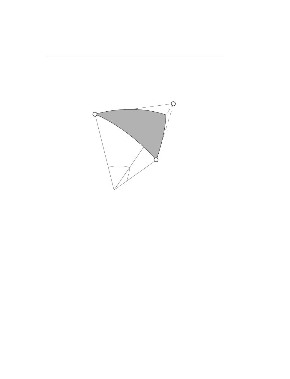
4.3 Mathematical model
69
are derived from the following formulae
d
TA(AI)
(t) = 2R
E
(R
E
+ alt (t)) 1 − cos ξ
TA(AI)
+ alt (t)
2
(4.8)
A
I
T
ξ
TA
ξ
AI
R
E
R
E
R
E
d
AI
d
TA
alt
Figure 4.2: Diagram that explains geometry used in 4.8
where R
E
= 6371 km
is the mean radius of the Earth, ξ
TA
and ξ
AI
correspond to great
circle arcs, measured in degrees and connecting the transmitter with the aircraft and the air-
craft with the receiver, respectively. alt denotes the altitude of the aircraft. Here, we assume
that both the transmitter T and the receiver I are within the visible horizon with respect to the
aircraft.
For each point from set U b
J
a
∗
,n
∗
we take every point from set U b
M
a
∗
,n
∗
and create trajectories
based on geodesics traversing through these points. These trajectories are then used to esti-
mate a family of synthetic Doppler curves by using (4.7) and compared against the curve f
e
.
The pair of two anchor points
ub
j,1
a,1
, ub
k,2
a,1
that produce the best fit is then used as reference
points for creating new sets of anchor points, as presented in 4.9
U
I
a,n
ub
1,1
a
∗
,n
∗
= ub
max(j
1
−1,1),1
a
∗
,n
∗
−1
(4.9a)
ub
g,1
a
∗
,n
∗
= ub
min(j
1
+1,g),1
a
∗
,n
∗
−1
(4.9b)
ub
1,2
a
∗
,n
∗
= ub
max(j
2
−1,1),2
a
∗
,n
∗
−1
(4.9c)
ub
g,2
a
∗
,n
∗
= ub
min(j
2
+1,g),2
a
∗
,n
∗
−1
(4.9d)
To clarify, in 4.9 we establish a new sets of points with location between two closest neigh-
bours of previously found points ub
j
1
,1
a
∗
,1
, ub
j
2
,2
a
∗
,1
. This step is repeated recursively, until the

70
4. Long-distance passive multi-static aircraft tracking
desired degree of precision is achieved. Let us denote the Doppler curve that corresponds
to the best fit after n
∗
= N
∗
iterations by f
b
and the estimated two sets of anchor points by
U b
I
a
∗
,n
∗
, n
∗
= N
∗
.
• Extrapolation. In order to find a trajectory for the region beyond the anchor points, we extrap-
olate the estimated trajectory using its characteristics, such as velocity and azimuth. Limits
for extrapolation are dictated by the previously defined time limits (t
I
l
, t
I
u
) and the velocity of
the aircraft.
4.4
Processing of an Experimental Data Set
In this section, we describe the data used to demonstrate the application of the mathematical model
presented above.
RSD was recorded by two receivers referred to by J
2
and M. In addition to RSD, we also retrieved
data from the web service http://www.flightradar24.com Flight Radar 24 (FR24) for
validation of model results.
The recording session for both sets of data (RSD and FR24) took place on July 12, 2012. The
spatial region that was taken to be the scope during FR24 recording encircles the southeastern
corner of Finland and the adjoining part of the Russian Federation. Data was retrieved from the
portal with a sampling rate of 10 s. However, the response from the portal was not immediate and
the sampling time thus varies. RSD was acquired with sampling rate of 2 MS/s. The receivers were
tuned to record spectrum of frequencies that includes transmitter frequency
(f
t
= 49.75 MHz)
and accompanying Doppler curves. Synchronisation with TV station was not required.
Locations of both receiving parties that were recording RSD J and M and the transmitting station T
are depicted in Fig. 4.5. The ERP of St. Peterburg’s TV station used in this experiment was 149 kW.
The antenna patterns that were used during the recording session include:
• for receiver J rotatable horizontal 4-element 50 MHz Yagi, gain about 5 dBd, height about 7 m
above ground, directive pattern typical to 5-element Yagis, and
• long wire of 250 m, which is slightly directional to northeast and has almost similar back lobe
pattern to south west, for receiver M.
The two baselines that join the positions of the receivers J and M with the transmitting station T are
denoted by b
J
and b
M
, respectively, and plotted as dashed lines. The map in Fig. 4.1 also displays
flight trajectories reconstructed from FR24 data. The flights are numbered with respect to the time
instances when they were discovered by the system within the defined region indicated in Fig. 4.1
by a dashed circle. Notable distances between receivers J , M , between receivers and the transmitter
J , S and M , S are respectively d
J,M
= 42.2 km, d
J,S
= 301.8 km, d
M,S
= 288.4 km.
A total of twenty four FR24 flights were recorded. From this set, three flights were classified to
group G1, namely, flights 3,10 and 11. Group G1 gathers flights which might have left Doppler
traces within RSD signals. We can notice that all the three trajectories end prematurely with respect
to the observed region. This is due to temporary lack of information on aircraft position from ADS-
B located in Joensuu, the eastern-most observation point on the flight corridors used by the flights.
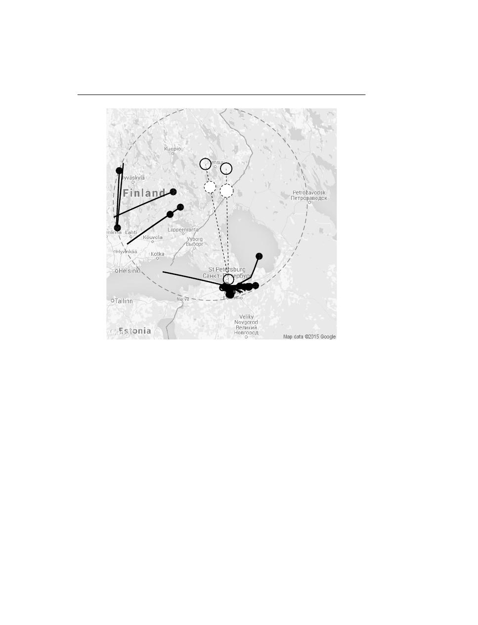
4.4 Processing of an Experimental Data Set
71
1
2
3
4
5
6
7
8
9
10
11
12
13
14
15
16
17
18
19
20
21
22
23
24
b
J
b
M
J
M
T
Figure 4.3: Map with recorded FR24 flight trajectories (solid black), locations of listeners J and M
and transmitter S together with two baselines b
J
and b
M
between the listeners and the transmitter.
RSD Doppler curve indicated with 1 in Fig. 4.4 that corresponds to FR24 trajectory 10 is taken as
an example of application of the system.
In this work we do not use any prior information on aircraft’s azimuth but we assume that an altitude
is constant for aircraft moving with cruising velocity and is equal to 11 000 m.
Fig. 4.4 presents spectrograms in the form of S
I
(t, ω
∗
) with frequency margin f
m
, f
m
= 199.22 Hz.
Here, on both RSD spectrograms, J and M, we can notice Doppler traces. The Doppler traces are
classified to be caused by the movement of three different aircraft. The approximate differences in
time between each pair of Doppler curves crossing the carrier frequency f
t
is equal to 2 min 14 s,
2 min 26 s and 2 min 27 s for Doppler curves 1 to 3 respectively. The Doppler curve crossing the
carrier frequency corresponds to the aircraft crossing baselines between the transmitter and the
receiver. Therefore, the deviation in time differences might come from different crossing locations
or different aircraft cruise speeds.
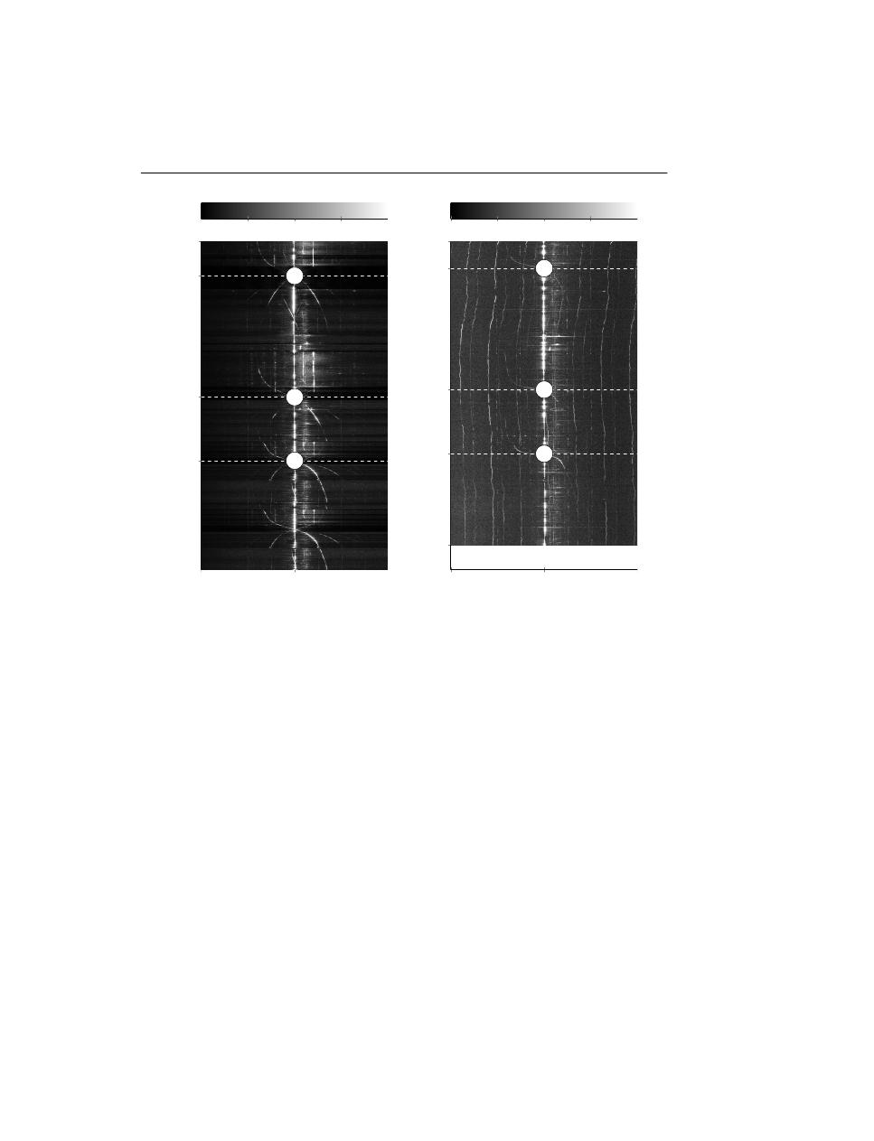
72
4. Long-distance passive multi-static aircraft tracking
-199.22
49750000
+199.22
19:52:05
20:27:20
20:47:51
21:27:03
21:38:08
1
2
3
-50
-39.9
-29.7
-19.6
-9.5
dB
-199.22
49750000
+199.22
19:52:05
20:00:04
20:29:34
20:50:17
21:29:30
21:38:08
1
2
3
-70
-58.1
-46.3
-34.4
-22.6
dB
Figure 4.4: Spectrograms for signals s
I
(t)
I={J,M }
together with marked three pairs of classified
Doppler curves. Horizontal and vertical axes are in Hz and wall clock units, respectively.
4.5
Case study
Among the pairs of Doppler curves presented in Fig. 4.4 we choose pair number 1 and consider it
as an example for the application of the mathematical model presented in the earlier section. The
next step involves setting lower and upper time limits t
l
, t
u
for the HT, as depicted in Fig. 4.5. The
lower and upper limits are set so that the visible RSD Doppler curve lies between them. Then the
Canny edge operator is applied to the limited part of the spectrograms and as a result we have a
binary representation (black and white) of the matrices S
I
(t, ω
∗
).
Next, the HT is used to extract segments of lines. Considering Doppler curves related to straight–
line–trajectories and the dimension of a pixel (cell of matrix S
I
(t, ω
∗
)) which is 0.5 s in the time
domain, or
1 Hz in the frequency domain, the angle parameter θ
I
is constrained to the interval
(−45
◦
, −1
◦
). The angle parameter should be smaller than −1
◦
to exclude the carrier signal from the
scope of the HT. The result of the HT is presented in Fig. 4.5 as segments of lines, together with the
first approximate crossing time t
x
I
.
Next, the segments that fulfil the conditions set by 4.5 are removed. After this, HT results are applied
for extracting Doppler curves from the spectrograms; this step is explained in detail in the descrip-
tion of the mathematical model. Extracted Doppler curves are depicted in Fig. 4.6, together with
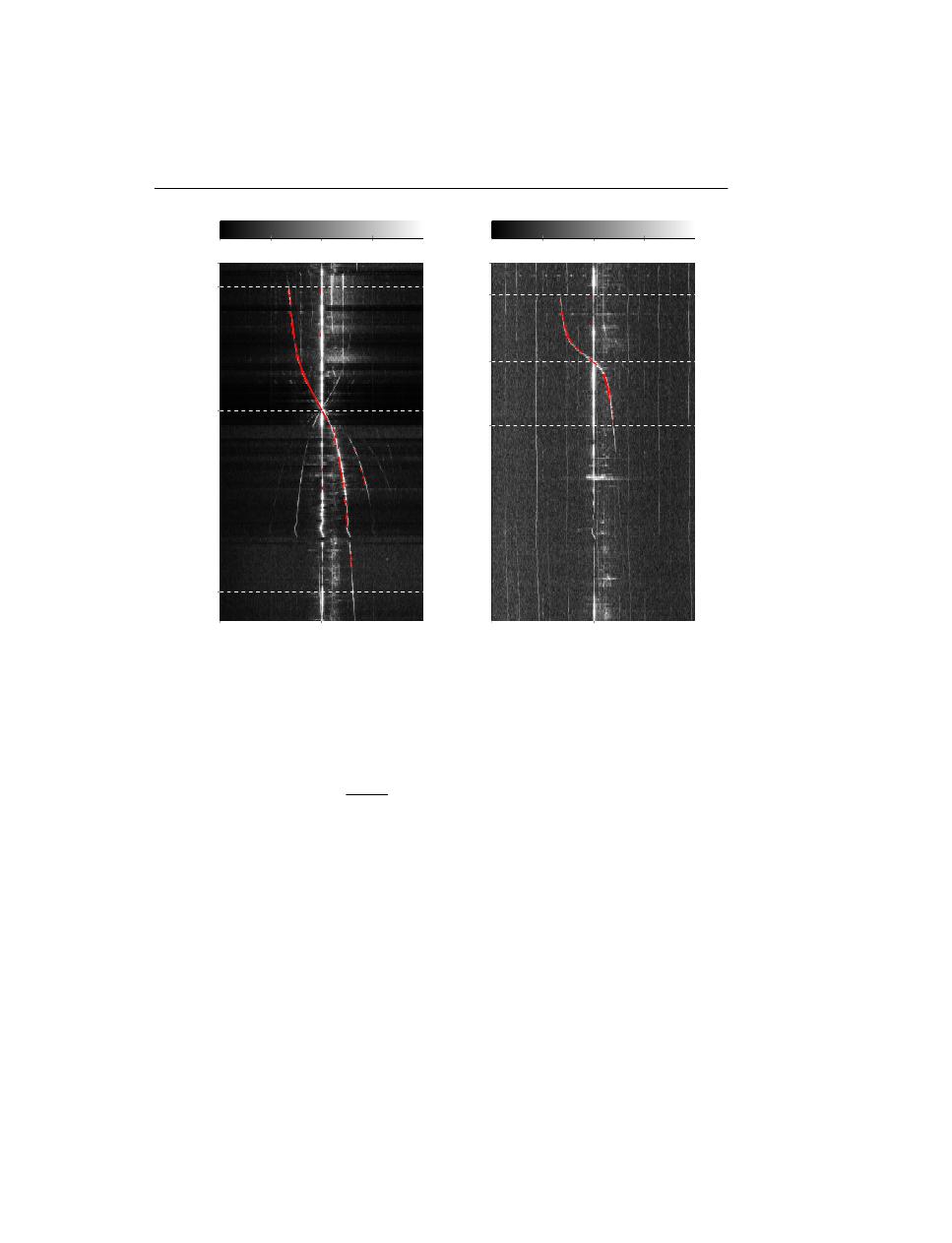
4.5 Case study
73
-199.22
49750000
+199.22
20:16:53
20:18:16
20:26:56
20:32:53
20:34:00
-50
-39.9
-29.7
-19.6
-9.5
dB
-199.22
49750000
+199.22
20:16:53
20:26:13
20:29:18
20:32:30
20:34:00
-70
-58.1
-46.3
-34.4
-22.6
dB
Figure 4.5: Results of the HT. The segments are depicted with red colour, time limits t
l
, t
u
– with
white dashed lines, crossing time t
x
I
– with white thick dashed lines.
the refined estimates of crossing time t
x2
I
. The differences between the first and second estimates
of crossing times are 6 s and 2 s for J and M, respectively. In that regard, the second approximation
might prove crucial for accurate aircraft trajectory estimation.
Fig. 4.7 presents results of the preliminary fitting. The trajectory that corresponds to the Doppler
curve for which the cost function f
e
− f
b
has the lowest value is presented on the map. The map also
includes marks for the anchor points (10 points). The points are located so that the full length of the
baselines and a distance of approximately 20 km beyond that is taken into account during the fitting
process. The spectrograms present the fit with cost function values equal to 0.314 Hz and 0.28 Hz
for J and M, respectively. As stated before in the mathematical model, the preliminary fitting is
based on finding the best anchor points. These anchor points correspond to crossing times in the
time domain. Therefore, the curves visible on spectrograms in Fig. 4.7 are limited by crossing times
t
x2
I
.
The preliminary fitting defines flight parameters, such as velocity, azimuth and location, with respect
to time. With this knowledge, we can extrapolate the trajectory beyond the baselines to meet the
condition t ∈ min t
I
l
, max t
I
u
. After this operation we once again calculate Doppler curves and
find the cost function which in this case equals 0.561 Hz and 0.635 Hz for J and M, respectively.
In Fig. 4.8, the extrapolated trajectory and corresponding Doppler curves are presented. The map
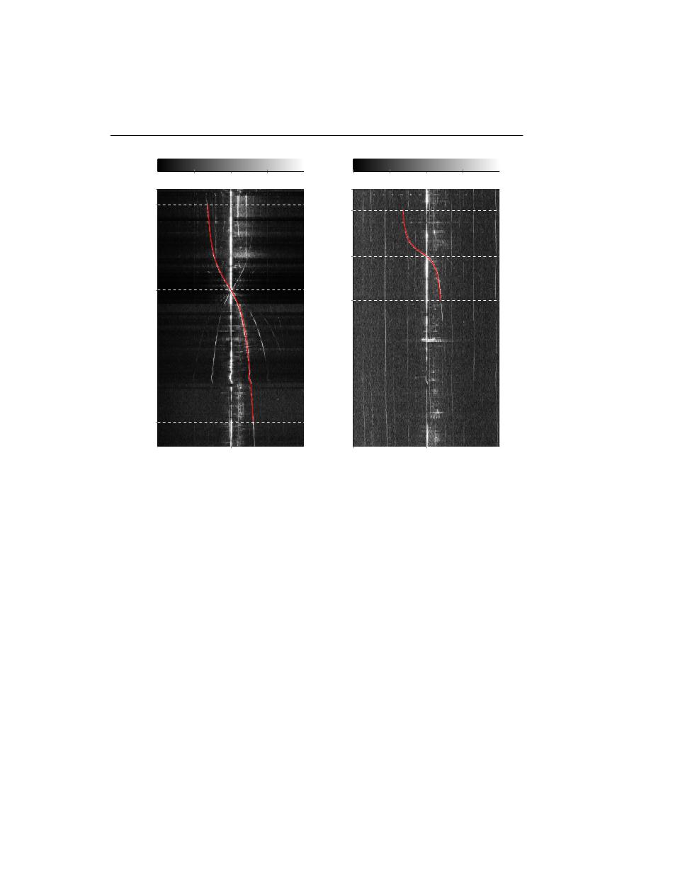
74
4. Long-distance passive multi-static aircraft tracking
-199.22
49750000
+199.22
20:16:53
20:18:31
20:27:02
20:32:58
20:34:00
-50
-39.9
-29.7
-19.6
-9.5
dB
-199.22
49750000
+199.22
20:16:53
20:26:37
20:29:17
20:32:35
20:34:00
-70
-58.1
-46.3
-34.4
-22.6
dB
Figure 4.6: Spectrograms with extracted RSD Doppler curves f
e
depicted with red solid lines.
Refine crossing times marked with white thick dashed lines.
also includes aircraft trajectories from FR24 for comparison. This trajectory is selected based on a
fine alignment between a synthetic Doppler curve and the estimated Doppler curve f
b
. Moreover, it
is shown how the Doppler curve f
b
prolongs the FR24 Doppler curve. However, we can notice that
the latter curve is quite noisy, when compared to the first one. Extrapolation of the FR24 trajectory
and its intersection with the two baselines b
I
results in deriving the location of two points l
I
. These
points are referred as to anticipated anchor points later in this section.
The fact that two trajectories, namely FR24 and estimated one, overlap over some portion of time is
used to show the spatial proximity between them. Fig. 4.9 presents results of comparing positions
of the two trajectories with respect to time. The location of the aircraft dictated by the estimated
trajectory slightly differs from the FR24. Moreover, the FR24 trajectory seems to wander around
the estimated trajectory. The flight speed is constant in the case of the estimated flight track which
is not the case with the FR24 record, probably because of lack of synchronizity between the various
clocks involved. The difference between their azimuths is 0.22
◦
.
The results demonstrate that the difference between positions of aircraft reconstructed with both
data sets vary between 200 m and 1600 m along the common flight trajectory. The difference across
the trajectory is less than 100 m.
Further analysis is conducted to ensure that the two sets of RSD data are properly synchronized
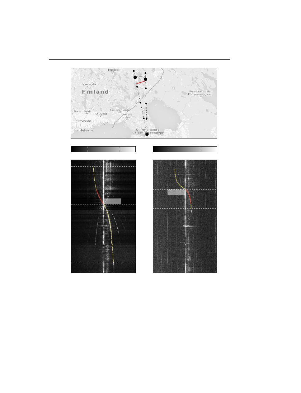
4.5 Case study
75
J
M
T
-199.22
49750000
+199.22
20:16:53
20:18:31
20:27:02
20:32:58
20:34:00
0.31401
-50
-39.9
-29.7
-19.6
-9.5
dB
-199.22
49750000
+199.22
20:16:53
20:26:37
20:29:17
20:32:35
20:34:00
0.28138
-70
-58.1
-46.3
-34.4
-22.6
dB
Figure 4.7: Results of preliminary fitting. Map: found trajectory with red solid line, anchor points
with small black marks. Spectrograms depict Doppler curves corresponding to the trajectory with
red colour. Yellow dashed lines depict previously extracted RSD Doppler curves f
e
.
with each other. This analysis shows that in the case of un-synchronized PC clocks between the two
listeners, which results in faulty relative start times t
0
I
, we are still able to determine the time shift
needed to synchronize the data. To detect the right time shift we perform a number of trajectory
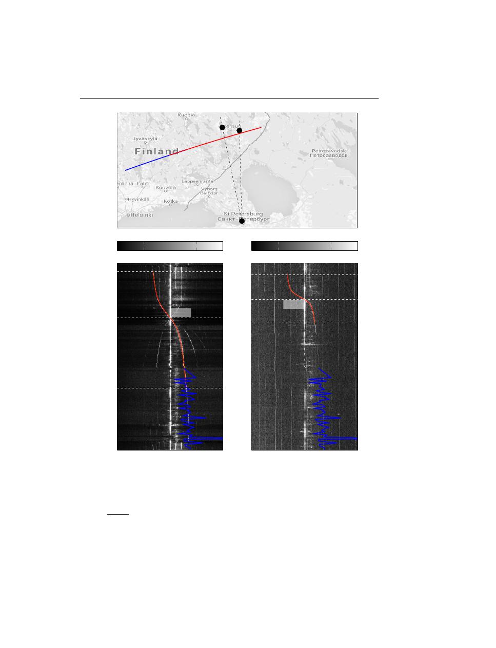
76
4. Long-distance passive multi-static aircraft tracking
J
M
T
-199.22
49750000
+199.22
20:10:53
20:18:31
20:27:02
20:32:58
20:34:00
0.561
-50
-39.9
-29.7
-19.6
-9.5
dB
-199.22
49750000
+199.22
20:10:53
20:26:37
20:29:17
20:32:35
20:34:00
0.635
-70
-58.1
-46.3
-34.4
-22.6
dB
Figure 4.8: Result of extrapolation: trajectory and corresponding Doppler curves – red colour. Blue
noisy curves on bottom pictures are Doppler curves resulted from recorded FR24 location/time data.
estimation runs with varying start time t
0
J
for listener J. During these runs we check the cost
function f
e
− f
b
and the distance from the anticipated anchor points l
I
to RSD-based anchor points
ub
I
a
∗
,n
∗
, n
∗
= N
∗
. Fig. 4.10 indicates that no time shift is needed for the data considered in this case
study.
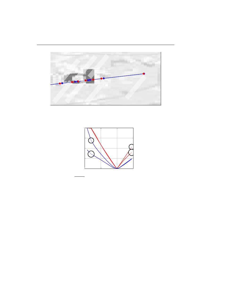
4.6 Discussion
77
20:18:43
1.
03
km
20:19:03
1.
35
km
20:19:13
0.
345
km
20:19:25
1.
121
km
20:19:38
1.
542
km
20:19:51
1.
033
km
20:21:00
0.
245
km
Figure 4.9: Region of overlapping trajectories of FR24 and estimated one. FR24 trajectory - blue,
the estimated trajectory - red marks. Pairs of connected marks depict locations for both trajectories
that correspond to the same time frames.
−40
−20
0
20
0.12
5.09
10.06
15.03
20
J
M
Distance
d
u
I
a,n
,l
I
,
n
=
N
km
−40
−20
0
20
0.56
3.56
6.55
9.55
12.55
J
M
Figure 4.10: Cost function f
e
− f
b
and distance d ub
I
a,n
, l
I
as a function of alternate start time t
0
J
.
Red lines corresponds to the left axis, blue to the right axis.
However, it shows that any time shift might cause a rapid change in the precision of the estimation
and a substantial growth in the distance from anticipated anchor points.
4.6
Discussion
In this work, we have developed a mathematical model for the estimation of the aircraft trajectory
based on Very High Frequency (VHF) frequency Doppler effect. With a heuristic method we clas-
sify Doppler curves visible from the spectrograms with respect to their relative position in time.
After a particular pair of Doppler curves has been selected for further analysis, the regions of the
spectrograms are restricted to a visible neighborhood of these Doppler curves. The Canny edge
operator is then applied to this region. As a result, edges in the spectrograms are detected. Next, we
find lines from the edge-detected-spectrogram with the Hough Transform (HT). The parameters for
the HT are set according to the resolution of the spectrogram image. The first estimate of the cross-

78
4. Long-distance passive multi-static aircraft tracking
ing time between the aircraft and the baseline connecting the transmitter and the receiver is derived
with the secant method. Outlying segments of the HT lines are then removed based on this estimate.
In the next step, Doppler curves from Radio Signal Data (RSD) spectrograms are extracted by using
the HT results and a smoothing technique.
The extracted curves are used as reference curves to which synthetically created Doppler curves
are fitted. The synthetic Doppler curves are created based on trajectories ensconced between anchor
points. The resulting trajectories are characterized by their cruise speed which is 900 km h
−1
±10 %.
The trajectory for which we found the best fit is then extrapolated with respect to its estimated cruise
speed and time limits.
For comparison we have used Flight Radar 24 (FR24) data to check the accuracy of the method.
The comparison brings out the following findings:
• the estimated trajectory is located relatively close to the FR24 one;
• the synthetic Doppler curve of the FR24 trajectory is considered to carry noise of significant
amplitude with respect to the estimated one, which is reflected in the precision of the trajectory
estimate.
The length of the estimated trajectory based on the extracted Doppler curves in our test case is
239 km and the initial distance between the aircraft and receiver J, for which the aircraft was track-
able, is 154 km. This fact makes the tracking method presented in this article comparable to that
obtained with other techniques. However, it should be emphasized that the method was tested under
favorable conditions regarding geographical location of receivers and the transmitter, Transmitter
Power Output (TPO), weather conditions, etc. Therefore, more tests are required to check its even-
tual efficiency and potential geographic span.
The final analysis tests the method for the case in which one (or more) reported RSD starting time
is inexact. Lack of synchronization between recording parties has to be considered as a possible
scenario. The analysis shows that the method is impervious to the time synchronization error.
Further development of the method might consist of enhancing the curve extraction method Wu and
Li (1996), as well as testing it over longer spatial distance between the aircraft and its observers.

C
HAPTER
V
Instantaneous Doppler signature extraction
Aircraft tracking based on the Doppler shift of radio sources of opportunity presents one approach
to avert or reduce tragedies like the lost flight MH370. Systems like this are based on simultaneous
observation of the Doppler shift caused by aircraft from multiple common radio sources and many
listeners, for example by capturing Doppler signals from spectrogram images. In the current article,
a mathematical model of instantaneous Doppler curve extraction from within a Very High Frequency
(VHF) spectrogram image is presented and exploited with three receiving and one transmitting
stations. The model is based on a priori knowledge of the probability density function of the first
order derivative of the Doppler shift, and on a system of blocks for identifying, classifying and
predicting the Doppler signal in a one-scan-at-a-time fashion. Tracing capabilities of such a model
are tested in an off-line experiment with twenty one TV signal recording sessions. The system was
able to trace 71 % of observed Doppler signatures; its stability was proven with various scenarios of
Doppler curve appearance within the recorded sessions and simulated synthetic data.
5.1
Introduction
Work presented in this publication is a continuation to the study on multi-static radar systems based
on Doppler-only information presented in Ptak et al. (2014) (Chapter 4). The previous paper de-
scribed the principles used for aircraft tracking by passive multi-static Doppler shifts. The system
was tested with Very High Frequency (VHF) recordings of Doppler footprints. This inverse prob-
lem of determining the location of the plane in spherical coordinates was approached by applying
a mathematical model consisting of a combination of the Hough Transform (HT), the Canny edge
detection operator and the secant method for minimization.
The present paper is meant to introduce a new method for extracting Doppler curves from within
the image (a spectrogram matrix). The spectrogram form as a signal representation provides ef-
ficient ways of analyzing it. In Thayaparan and Kennedy (2004) authors present advantages and
disadvantages of different time-frequency representations in a manoeuvering air target scenario.
The spectrogram representation which is pursued in this paper is designed to be quickly executable
without any major loss of resolution. The method presented focuses on commercial aircraft detec-
tion, with the lost flight MH370 as a reference scenario, in which case the trajectory of the aircraft
tends to follow geodesics with some minor bends. The approach used here differs from the one pre-
sented in the previous paper Ptak et al. (2014) by the instantaneous identification of Doppler curve
79

80
5. Instantaneous Doppler signature extraction
components. The mathematical model consists mainly of Cell Averaging – Constant False Alarm
Rate (CA-CFAR), signal intensity analysis and signal crossing scenario analysis.
In Xiangwei et al. (2003) several Constant False Alarm Rate (CFAR) techniques suitable for over-
the-horizon reception are tested. CA-CFAR is chosen over the other techniques tested in order to
get good signal detection. However, in a multiple target scenario the Clutter Map – Constant False
Alarm Rate (CM-CFAR) or the Trimmed Mean – Constant False Alarm Rate (TM-CFAR) methods
would perform better in recognizing interfering targets according to these authors.
In Li et al. (2012) the authors present an approach to detect Doppler signatures of human movements
micro–Doppler (µD) and classify them into separate categories. For feature extraction the authors
proposed applying a smoothing median filter over the computed maximum power spectrum and then
applying two techniques, namely a Two-directional Two-dimensional form of Principal Component
Analysis (2D2-PCA) and Two-directional Two-dimensional form of Linear Discriminant Analysis
(2D2-LDA).
The idea of detection of components within a spectrogram is a well-studied subject. Some exam-
ples involve harmonic component tracking in audio signals with a sequential Bayesian harmonic
model (Dubois and Davy, 2007), using Fractional Spectrograms (FS) to compute the Instantaneous
Frequency (IF) of multicomponent nonstationary signal Khan and Boashash (2013), separation of
a percussive component containing transients as an application of Time-Scale Modification (TSM)
Driedger et al. (2014), human fall detection using time-varying Doppler signatures analyzed with
time-frequency representations and matching pursuit decomposition Wu et al. (2013). In Khan and
Boashash (2013) the authors have demonstrated method for multicomponent signal separation using
an adaptive window fractional spectrogram provided that the local amplitudes of signal components
do not vary significantly, whereas this publication presents a separation method based on separate
peak recognition (mass regrouping). This method was chosen over a maxima detection based one
in a past study of extraction of Frequency Modulation (FM) based signal Djurovi´c and Stankovi´c
(2004).
In Plante et al. (1998) the authors demonstrate a Method of Reassignment (RM) in which at every
time step scattered components are reallocated on a time–frequency plane to a new point that rep-
resents the distribution of energy in the time–frequency window more accurately. A special case
of reassignment was introduced in Daubechies and Maes (1996) as a Synchrosqueezing Transform
(SST) which the purpose of identifying speakers by incorporating a wavelet transform and auditory-
nerve based models. In contrast to reassignment transform the SST allows for mode reconstruction
(more efficient mode separation than Empirical Mode Decomposition (EMD)). A comprehensive
overview of these two methods (RM and SST) is presented in Auger et al. (2013). In the present
paper however the components are not shifted on the plane but rather followed as they are located
with respect to their center of mass. In other words the current method allows the signal to locally
fluctuate on the plane while still being trackable.
Connecting the detected components at different time instances is a well-studied subject. The
Viterbi Algorithm (VA) has been tested in different fields of interest Hara et al. (1997); Ochiai
(2004); Djurovi´c and Stankovi´c (2004). The concept of the VA has been used in this paper, but the
idea behind the current algorithm does not match fully the specifics of VA, see section 5.3.5.
The paper is organized as follows. After the current Introduction, the second section covers the
fundamentals for the ensuing analysis which is derived from the probability density function (PDF)
of the first order derivative of Doppler shift (FODDS). The third section introduces the mathematical

5.2 PDF of FODDS with respect to varying sampling time and cruising velocity
81
model developed here. In the fourth section a description of the recording circumstances and the data
recorded and simulated are presented. Experimental results with the proposed model are presented
in section five. Discussion of the results is presented in section six.
5.2
PDF of FODDS with respect to varying sampling time and cruising ve-
locity
Let us start from the well known bistatic Doppler shift equation presented in (5.1).
f
D
(t) =
f
t
c
d (d
TA
(t) + d
AI
(t))
dt
(5.1)
where f
t
represents the transmitted frequency, d
TA
(t) and d
AI
(t) are distances from the transmitter
to an aircraft and from an aircraft to the receiver, respectively; c is the speed of electromagnetic
waves and f
D
(t) corresponds to the Doppler frequency (shift), I = J, M.
Distances d
TA
(t) and d
AI
(t) from (5.1) can be expanded into the following form
d
TA
(t (1)) =
(x − x
T
)
2
+ (y − y
T
)
2
(5.2)
d
TA
(t (2)) =
(x + ∆x − x
T
)
2
+ (y + ∆y − y
T
)
2
(5.3)
d
TA
(t (3)) =
(x + 2∆x − x
T
)
2
+ (y + 2∆y − y
T
)
2
(5.4)
where x and y are constrained to the following domain [−0.7d
TR
, 0.7d
TR
] × [−d
TR
, d
TR
], t (3) =
t (2) + T = t (1) + 2T , d
TR
– length of the baseline, (x
T
, y
T
) – transmitter location, (x
R
, y
R
) –
receiver location, ∆x = V
c
T cos γ, ∆y = V
c
T sin γ. Parameter γ is an angle between the receiver-
transmitter vector and the vector of the object’s trajectory, measured counterclockwise, see Fig.
5.1. Two of the remaining parameters V
c
and T are the cruising velocity and the sampling time,
respectively.
Sequence d
AI
(t (1)) . . . d
AI
(t (3)) has a similar construction.
Substituting the bistatic distance at time t (p), d
TA
(t (p)) + d
AI
(t (p)) with d
b
(t (p)) gives (5.1) a
discretized form
f
D
(x, y, γ, T, V
c
) =
f
t
c
d
b
(t (p − 1)) − d
b
(t (p))
T
(5.5)
Therefore the first derivative of (5.5) can be expressed as follows
∂f
D
(x, y, γ, T, V
c
)
∂t
=
f
t
c
d
b
(t (p − 2)) − 2d
b
(t (p − 1)) + d
b
(t (p))
T
2
(5.6)
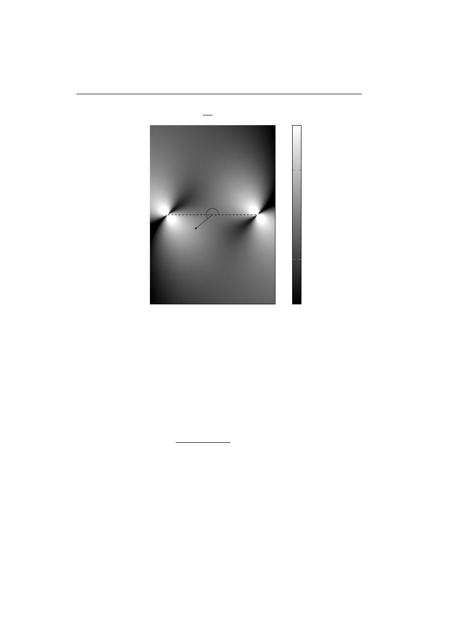
82
5. Instantaneous Doppler signature extraction
−0.7d
TR
0.7d
TR
−d
TR
d
TR
T
R
γ
x
y
∂f
D
∂t
dB
-2.1
-1.08
-0.07
0.95
1.97
Figure 5.1: A graph of the first derivative of the Doppler shift with respect to spatial variables x and
y and constants T = 0.5 s, V
c
= 250 m s
−1
and γ = 220
◦
.
An example of the distribution of the first derivative of the Doppler shift as a function of spatial
location is presented in Fig. 5.1. In this case the angle γ is set to 220
◦
, cruising velocity V
c
=
250 m s
−1
and sampling time T = 0.5 s.
The Probability Density Function (PDF) of the First Order Derivative of Doppler Shift (FODDS)
value as a function of cruising velocity V
c
and sampling time T is expressed as
Pr [V
c
, T ] =
π
0
d
TR
−d
TR
0.7d
TR
−0.7d
TR
∂f
D
(x, y, γ, T, V
c
)
∂t
dxdydγ
(5.7)
An interesting phenomenon can be observed in Fig. 5.2. As the cruising velocity increases, the
limits of PDF’s domain (the first derivative) shift towards higher values. However the changes are
not large which can be seen from Fig. 5.3 which demonstrates the change in the first derivative with
the highest probability value over varying cruising velocity.
The graph in Fig. 5.4 depicts the PDF presented in (5.7).
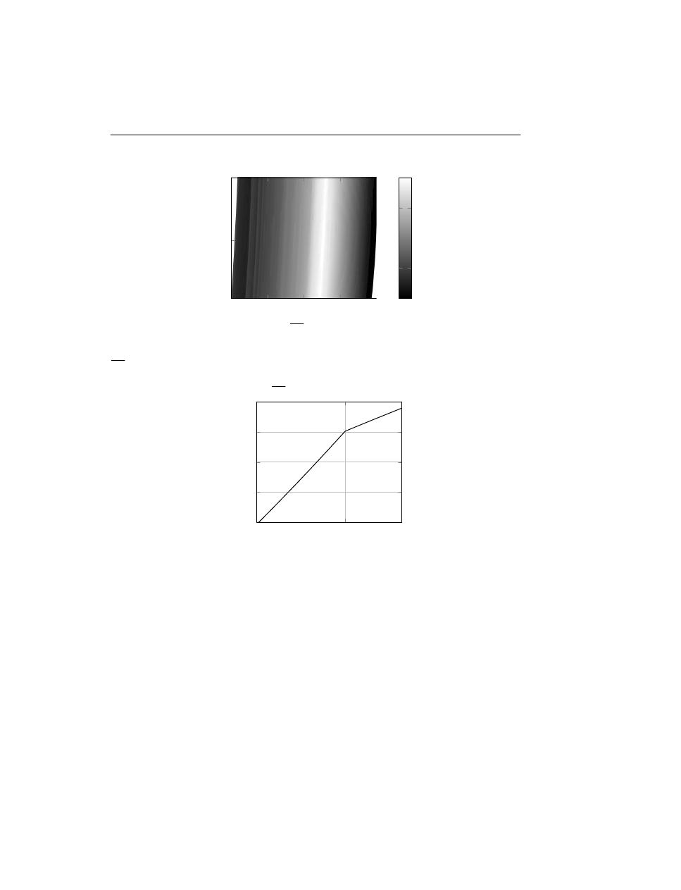
5.3 A Doppler curve detection model based on PDF of FODDS
83
10
−7.21
10
−4.86
10
−2.51
10
−0.16
10
2.19
190
245
305
∂f
D
∂t
Hz
V
c
m
s
−
1
Pr [V
c
, T ] dB
-7.27
-5.63
-3.99
-2.35
-0.71
Figure 5.2: Graph of PDF of FODDS value Pr [V
c
, T ] as a function of aircraft cruising speed V
c
and
∂f
D
∂t
.
190
260
305
3 · 10
−2
4 · 10
−2
5 · 10
−2
6 · 10
−2
7 · 10
−2
V
c
m s
−1
∂f
D
∂t
Pr[V
c
,T ]=max(Pr[V
c
,T ])
Hz
Figure 5.3: FODDS as a function of cruising velocity V
c
for maximum observed probability.
5.3
A Doppler curve detection model based on PDF of FODDS
In this section a mathematical model of Doppler curve detection is presented. It is assumed that
the system is incapable of tracing Doppler curves that emerge from isorange contour trajectories, or
baseline’s trajectory.
The model consists of the following blocks:
• Cell Averaging – Constant False Alarm Rate (CA-CFAR) model. It is used to scan in line-
by-line pattern in order to detect cells with amplitude over a certain threshold, that with some
certain probability corresponds to the target echo.
• Cells detected with CA-CFAR are analyzed to find separated peaks, defined as a group of
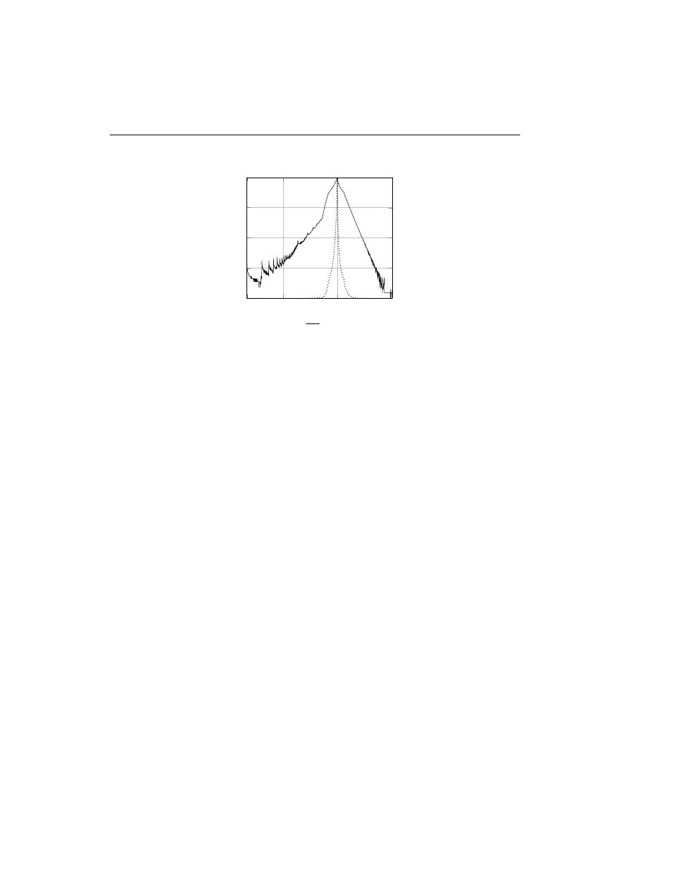
84
5. Instantaneous Doppler signature extraction
10
−7.01
10
−4.71
10
−1.29
10
2.2
0
5.8 · 10
−3
1.17 · 10
−2
1.75 · 10
−2
2.33 · 10
−2
∂f
D
∂t
Hz
Pr [V
c
, T ]
−2.5357
−2.2347
−1.9337
−1.7576
−1.6326
Figure 5.4: Probability Density Function of FODDS. The dotted line corresponds to linear scale
(left axis), whereas the solid to logarithmic one (right axis).
neighboring points corresponding to the same peak, which could represent different signal
sources. This step is achieved through analysis of first and second derivatives.
• The Center of Mass (CoM) formula is applied to find the frequency that corresponds to the
true maximum amplitude of each peak. The maximum-amplitude frequency points thus found
are then named as the pretenders.
• To aid prediction of the forthcoming position of signal in frequency domain we calculate the
expected value of ∂f
D
(x, y, γ, T, V
c
) /∂t and denote it with E [∂f
D
/∂t], see section 5.3.5.
• Classification block in which the system classifies the pretenders into separated groups which
form a logically consistent time series in a sense of Doppler shift curvature. The Classification
block is mainly based on a continuation of the energy concentration parameter, the distance in
frequency between two consecutive steps and probability Pr [V
c
, T ] of frequency difference.
• Signal intersection block is responsible for finding cases in which two or more signals are
intersecting for some period of time. It solves these cases by predicting and separating the
signals based on the history of the signal’s shape and amplitude.
• Rejection block consists of the set of rules needed to reject or accept the pretenders’ group.
• Prediction block is based on a first or second order polynomial fit of the groups of the pre-
tenders found, depending on the class of the signal, and on an extrapolation one step (one
scan line) forth.
• Linking block is responsible for joining two signals separated by a time gap once certain
conditions are fulfilled.
Each of the listed blocks and interactions between them is presented in Fig. 5.5 and in the forthcom-
ing subsections.
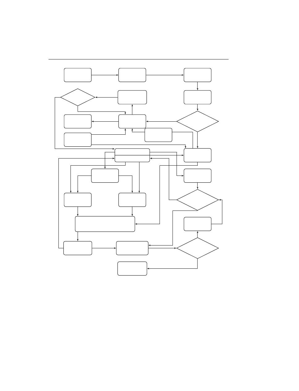
5.3 A Doppler curve detection model based on PDF of FODDS
85
Spectrogram’s
row
CA-CFAR
(5.3.1)
Grouping
(5.3.2)
IF
e − s > n
s
Center of mass
(5.3.3)
Matching groups
(5.3.5)
IF
condition (5.23)
Matrix M
(5.3.5)
Matrix M
(5.3.5)
New sequence
Continuing sequence
Discarded
(5.3.5)
Prediction
back
Classification
(5.21)
IF
condition (5.24)
Carrier
Doppler
Prediction
forth
• Predicition/new groups comparison
• Quality measures assigned–(5.20)
• Intersection of D–C,D–D, (5.3.6)
IF
condition (5.25)
Termination rule
(5.22)
Temporarily stored
sequences
Stored sequences
FODDS
(5.3.4)
N
Y
N
Y
N
Y
N
Y
Remaining
cells of M
Figure 5.5: Organigram of procedure presented in section 5.3
5.3.1
Cell Averaging – Constant false alarm rate
Let us denote a matrix of spectrogram data by S
I
[n×m]
and an amplitude of each cell of this matrix by
S (t (p) , ω (j)), where t (p) , p ∈ [1, n] denotes a time for the cell being measured, and ω (j) , j ∈
[1, m] a frequency that corresponds to the cell.

86
5. Instantaneous Doppler signature extraction
To check if detection is found in Cell Under Test (CUT) we need to check the equation 5.8
S (t (p) , ω (j)) > k
CF AR
1
n
RC
j∈RC
S (t (p) , ω (j))
(5.8)
where RC denotes a reference cell’s location in the frequency domain and is of length n
RC
, k
CF AR
stands for a scaling constant. If the inequality is satisfied then CUT is stored and denoted as
S (t (p) , ω (j
i
, t (p))) , j
i
∈ [1, m].
5.3.2
Grouping
The points found in the previous step are now grouped to form separate peaks of signals. This
separation is achieved by examination of the frequency distance between them. If
ω (j
i
, t (p)) − ω (j
i+1
, t (p)) < f
mr
,
(5.9)
where f
mr
denotes the frequency margin between two points, then it is said that S
H
(t (p) , ω (j
i
, t (p)))
and S
H
(t (p) , ω (j
i+1
, t (p))) belong to the same group (set) H, and i, i + 1 ∈ [1, |H|], |H| denotes
the cardinality of the group (set) H. Further it is assumed that each group corresponds to a separated
signal, both those desired to be discovered, like Doppler curves, and those originating in another
source.
5.3.3
Center of mass
The aim of this step is to find the Center of Mass (CoM) (gravity) of previously established groups.
In this case mass corresponds to the amplitude of each cell S
H
(t (p) , ω (j
i
, t (p))) and its location
is measured relative to the frequency ω
H
(j
i
, t (p)). For group H of cardinality equal to b
H
this is
achieved through the following formulae in (5.10) and (5.11).
ω
l
(t (p)) =
1
N
w
b
H
i=1
[S
H
(t (p) , ω (j
i
, t (p))) ω
H
(j
i
, t (p))]
(5.10)
a
l
(t (p)) = S
H
(t (p) , ω
l
(t (p)))
(5.11)
where N
w
=
b
H
i=1
S
H
(t (p) , ω (j
i
, t (p))). A pair (ω
l
(t (p)) , a
l
(t (p))) denotes frequency and ampli-
tude of the center for group H at time t (p). The value of the amplitude refers to an interpolated
value between amplitudes of two closest neighbors. The found pairs (ω
l
, a
l
) are then referred to as
pretenders
for signal carrying cells. Let us denote a number of pairs (pretenders) (ω
l
, a
l
) detected
at time t (p) as q (t (p)).

5.3 A Doppler curve detection model based on PDF of FODDS
87
5.3.4
Expected value
To aid the prediction of the position of a pretender in a next scan S (t (p + 1)) we use the previously
established PDF of the FODDS glsprobdist [V
c
, T ]. The expected value E [V
c
, T ] is used to predict
the location of the next pretender for some given group H when there is not enough historical data
(length of a set S
H
(t (p) , ω (j
i
, t (p))) in time domain is limited to a couple of scans) on which
proper prediction could be based. Let us denote the length of the signal that is needed for predicting
its next frequency value (location within frequency spectrum ω) by n
h
.
5.3.5
Classification and prediction
Classification block is the most important part of the system. It allows continuous monitoring of a
previously detected pretender. The efficiency of classification depends on the quality of the signal,
measured by its Signal to Noise Ratio (SNR), gaps in signal reception, etc.
With every new scanned line we need to conduct a number of calculations. The first of these
(5.12) is to check every pair of newly found pretenders and pretenders from the previous scan
for their frequency differences. The resulting parameter is the first out of four that will control
classification and determine how the sequence of matching pretenders eventually forms a signal.
All four parameters are represented in the form of matrices.
l1∈[1,q(t(p−1))]
l2∈[1,q(t(p))]
F
l1,l2
(t (p)) = ω
l1
(t (p − 1)) − ω
l2
(t (p))
(5.12)
The second parameter is a result of constraining frequency differences obtained from (5.12) and its
boolean values F
m
l1,l2
can be evaluated from (5.13)
l1∈[1,q(t(p−1))]
l2∈[1,q(t(p))]
F
m
l1,l2
(t (p)) = |F
l1,l2
(t (p)) < f
mr
|
(5.13)
The next parameter determines energy concentration for each group and then checks for multiplica-
tion of energy concentration for each group from the previous step with each group from the present
step. The following formula (5.14) represents the energy concentration value ec for group H of
cardinality b
H
:
ec
l
(t (p)) =
b
H
i=1
S
H
(t (p) , ω (j
i
, t (p)))
ω
H
(j
b
H
, t (p)) − ω
H
(j
1
, t (p))
(5.14)
The third crucial parameter, EC
l1,l2
, is obtained by the following formula (5.15).
l1∈[1,q(t(p−1))]
l2∈[1,q(t(p))]
EC
l1,l2
(t (p)) = ec
l1
(t (p − 1)) · ec
l2
(t (p))
(5.15)

88
5. Instantaneous Doppler signature extraction
The fourth parameter uses knowledge on probability distribution of the FODDS
l1∈[1,q(t(p−1))]
l2∈[1,glsnumpret(t(p))]
P
l1,l2
(t (p)) = Pr [V
c
, T ]
∂fD
∂t
=F
l1,l2
(t(p))
(5.16)
Two of the aforementioned parameters are then normalized by the following equations (5.17,5.18).
l1∈[1,q(t(p−1))]
l2∈[1,q(t(p))]
F
s
l1,l2
(t (p)) =
1
1 + |F
l1,l2
(t (p))|
(5.17)
l1∈[1,q(t(p−1))]
l2∈[1,q(t(p))]
EC
s
l1,l2
(t (p)) =
EC
l1,l2
(t (p))
max (EC
l1,l2
(t (p)))
(5.18)
For the sake of simplicity, notations for the four established parameters are: F
s
for normalized
frequency differences matrix, F
m
for the matrix of frequency differences in a logical form, EC
s
for
the matrix of normalized energy concentration and P for matrix of the probability distribution. The
four aforementioned parameters are then combined in the following fashion
M = F
s
◦ F
m
◦ EC
s
+ P
(5.19)
where the operator ◦ denotes the Hadamard product. The newly established matrix M is a measure
of the quality of matching between groups from the previous scan and those from the present one.
The next step is to iteratively check matrix M for cells with highest values. Once the highest value
has been found, let us denote the corresponding cell with mt
l1,l2
. Then the cells in the corresponding
row l1 and column l2 are zeroed. In other words, this step allows only one to one relations between
groups. This is repeated until the null matrix form is achieved.
Estimation of matrix M is repeated for each progressing scan. If during the process of selection
by operation on matrix M one (or more) of the groups is consecutively chosen n
s
times to have
continuation in the next scan then the sequence of ’matching’ groups is considered as a potential
signal. The sequences that do not reach the length of n
s
are rejected and considered useless for
further analysis. Let us denote the sequence l as w
l
(t [st, en]), where st and en denote scan numbers
when the sequence started and ended (or present scan), respectively.
Once the sequence is formed the system initializes prediction to anticipate frequency value one
scan ahead. The prediction is based on the last n
h
historical frequency values fitted with a second
order polynomial. In some cases the system uses a first order polynomial, see section 5.3.6 for
details. Parameter n
h
varies depending on the actual length of the sequence and can be defined as
n
h
= min {n
s
, n
hu
} where n
hu
denotes an upper limit for the parameter n
h
.
To distinguish the present quality of the signal (at time t (p)) it is crucial to attribute a quality
measure
h
l
(t (p)) ,
(5.20)

5.3 A Doppler curve detection model based on PDF of FODDS
89
to a sequence l. It is done by checking if any of the newly found groups are within estimated
prediction boundaries. If there exists a group that satisfies this condition then h
l
(t (p)) = 1, if not
then zero is assigned.
The sequence is then categorised into two groups, the first one corresponding to a Doppler-related-
signal (D) and the second one to a carrier-related-signal (C). The condition for a carrier-related
signal is defined in (5.21)
(p = n
c
∧ |p
l
(t (1)) − p
l
(t (p))| < f
mc
) ⇒ w
l
= w
c
l
(5.21)
where the pair (n
c
, f
mc
) are a length of the sequence w
l
for which we check if its trend (first order
polynomial fit) p
l
has deviated by f
mc
from its starting frequency value, w
c
l
denotes a newly classi-
fied sequence as a carrier (hence superscript c). The sequences that do not satisfy this condition are
classified to be Doppler related.
If the signal fades out then for some time there are no recognized groups within prediction bound-
aries and therefore the prediction itself is used as a new estimation. In this case the assigned quality
measure equals zero. If the vector of quality measure satisfies the following condition
1
n
s
p
i=p−n
s
+1
h
l
(t (i)) < p
tr
(5.22)
then the signal is terminated and temporarily stored.
5.3.6
Intersection of sequences
This section explains the case when two or more sequences intersect on the frequency-time plane
(spectrogram). Examples of intersection might involve two (or more) Doppler sequences (D-D)
or Doppler and carrier sequences (D-C). In the latter case the carrier sequence tends to behave as
stationary frequency-wise, but it can, and occasionally does, sway due to different equipment and
weather related causes.
For this part of the mathematical model, we assume that the sequence w
l
exists
l∈Z
(w
l
∨ w
c
l
)
(5.23)
and is longer than n
s
(en − st + 1 > n
s
) and prediction is initialized. Among cells of matrix M we
choose those that correspond to sequences longer than n
s
. From this set we choose the one with the
highest value and proceed by checking if its value is positive (> 0). If that is the case then we store
it for further analysis as w
x
l
.
The stored sequences w
x
l
are now analyzed for a possible intersection scenario. A condition that
needs to be fulfilled is that two (or more) sequences share the same column of matrix M. In other
words two (or more) sequences point at the same group as the continuation. Then depending on
sequence category we use a different prediction. In the case of a Doppler signal we use a second
order polynomial to estimate the next element of the sequence, for carrier sequences we use a first
order polynomial with a significantly longer history tail on which the next element is estimated. In
both cases the quality measure h
l
(t (p)) = 1.

90
5. Instantaneous Doppler signature extraction
5.3.7
Combining sequences
This step is important as a backup solution in a case when the system lost trace on some signal.
Because situation like that is possible we need to implement a solution for combining two curves
where one of them mathematically prolongs the other one.
Every time when the new signal has been formed the system checks whether it is a continuation
of any of the previous terminated signals or not. For every pair of present w
l
and past w
z
signals
the prediction to past and prediction to future are performed, respectively, with length of prediction
n
l,z
matching the time gap between them. Once the results of prediction f
l
(t [st − n
l,z
, st − 1]),
f
z
(t [en + 1, en + n
l,z
]) are known the system checks the following condition:
n
l,z
i=1
ω
l
(t [st − i]) − ω
z
(t [en + n
l,z
− i + 1]) < n
l,z
f
mrp
(5.24)
where f
mrp
is a frequency margin for predicted values. If the condition is fulfilled then the sig-
nals are joined and the gap is complemented with values resulting from fitting the subsequences
ω
z
(t [en − n
s
, en]) and ω
l
(t [st, st + n
s
− 1]). If the condition is not met then the system recog-
nizes the present signal as a completely new one. Selection of potential past signals is made based
on condition of time difference
t
l
(st) − t
z
(en) < t
p
,
(5.25)
where t
p
is a time margin for the potential signal.
5.4
Data set specification
5.4.1
Recorded sessions
This section describes the data set used to demonstrate the application of the mathematical model
presented in section 5.3.
The Radio Signal Data (RSD) was captured by three receivers, J
1
, J
2
and M located near Joensuu,
Finland. Receivers J
1
and J
2
corresponds to the same geographical location but different antenna
configurations. A TV station located in Saint Petersburg, Russian Federation was used as a trans-
mitter of opportunity. The receiving antennas’ parameters were as follows:
• 4-element horizontal dipole array at about 14 m above ground, with dipole end dip directed to
Saint Petersburg transmitter to attenuate signal strength increase during carrier crossing, for
receiver J
1
,
• rotatable horizontal 4-element 50 MHz Yagi, gain about 5 dBd, height about 7 m above ground,
directive pattern typical to 5-element Yagis, for receiver J
2
and
• long wire of 250 m, which is slightly directional to northeast and has almost similar back lobe
pattern to south west, for receiver M.

5.4 Data set specification
91
The recording sessions of RSD took place on July 12, 2012 with use of J
2
and M receivers and
within March 22 to April 26, 2014 with use of J
1
and J
2
receivers.
RSD was acquired with sampling rate of 8 kHz. The receivers were tuned to record a spectrum of
frequencies that includes the transmitter frequency (f
t
= 49.75 MHz) and accompanying Doppler
curves. To obtain spectrogram form of RSD Bracewell (2000) the Short Time Fourier Transform
(STFT) was used with the width of symmetrically positioned Hann window set to L ∼ 1 s, (8192
samples) and calculation time step to G = 0.5 s. With these settings the spectrogram is categorized
as overlapped with overlapping time of ∼ 0.5 s. This window specification ensures that information
on the signal’s magnitude is not lost (Izraelevitz, 1985). Moreover half a second time resolution
combined with 8192 samples per window provides a good time/frequency resolution for the Doppler
signature of common length of tens of minutes. By studying PDF of FODDS we can deduce that
0.5 s window will in most cases be sufficient to ensure steady and traceable transition of Doppler
signature in frequency domain, discarding some extreme cases such as aircraft trajectories passing
through the baseline or nearly parallel to it.
Locations of both receiving parties that were recording RSD (J and M) and the transmitting station
(T) are depicted in Fig. 5.6. The Effective Radiated Power (ERP) of St. Peterburg’s TV station used
in this experiment was 149 kW.
d
TJ
d
TM
d
JM
J
M
T
Figure 5.6: Geographical location of transmitter T and receivers J, M and distances between them.
92
5. Instantaneous Doppler signature extraction
Notable distances between receivers J, M, between the transmitter T and receivers J, M, are respec-
tively d
JM
= 42.2 km, d
TJ
= 301.8 km, d
TM
= 288.4 km.
Fig. 5.7 presents an example of recorded data in a form of spectrograms. In this case RSD comes
from simultaneous recordings from J
1
and J
2
. It is worth to mention that the signatures received
with J
1
are noticeably longer but also have a lower SNR.
-84.9
49750000
+84.7
13:20:27
13:55:27
14:30:27
15:05:27
15:40:28
ω Hz
J
1
, 2014-04-26
-84.9
49750000
+84.7
13:20:27
13:55:27
14:30:27
15:05:27
15:40:28
ω Hz
J
2
, 2014-04-26
Figure 5.7: Example of recorded Doppler signatures. The receivers J
1
and J
2
were tuned to receive
signal from the same transmitter T.
5.4.2
Simulated signal
To complement the experimental part the synthetic Doppler signal was simulated with help of
Phased Array System Toolbox
TM
being a part of MATLAB
TM
. The scenario of this simulation
was suppose to imitate conditions presented in section 5.4.1. The length of the baseline was set
to d
TR
= 301 km, location of the transmitter was set at the origin (0, 0, 0), receiver’s location
to (0, d
TR
, 0). Aircraft starting st and finishing f i location was chosen randomly as A
st
(x, y) =
{U (−0.6d
TR
, −0.2d
TR
), U (−0.2d
TR
, 1.2d
TR
)}, A
f i
(x, y) = {U (0.2d
TR
, 0.6d
TR
), U (−0.2d
TR
, 1.2d
TR
)},
and so was the altitude alt = U (9750, 11270)m and the velocity V
c
= U (244, 257)m s
−1
.
The transmitting frequency f
t
remained the same as in the case of St. Petersburg TV station. To
obtain a different SNR of resulting Doppler signal the power of transmitted signal varied as P
av
=
U (0, 100)W.

5.5 Case Study
93
The simulation involved three statistical models for the target’s Bistatic Radar Cross Section (BRCS),
namely: Nonfluctuating, Swerling 1 and Swerling 2; additionally an ogive model was simulated and
represented by equation (5.26) for ogive’s BRCS Siegel et al. (1955), over which the Swerling 2
model was added to simulate smaller fluctuations.
σ
a
=
λ
2
tan
4
ϕ (1 − tan
2
ϕ tan
2
(β/2))
−3
16π cos
3
(β/2)
,
(5.26a)
0 ≤ β < π − 2ϕ
πL
2
o
(sin (β/2) − cos ϕ)
4 sin
2
ϕ sin (β/2)
,
(5.26b)
π − 2ϕ < β < π
where λ, ϕ, β and L
o
denotes wavelength, half angle, bistatic angle and ogive’s length, respectively.
Additionally rectangular FM signal was used as a transmitted signal. Parameters characterizing the
transmitting/reflecting/receiving ends were as follows:
• transmitting frequency f
t
= 49.75 MHz
• sampling frequency f
s
= 15 kHz
• pulse width = 1/1500 s
• Pulse Repetition Frequency (PRF) f
p
= 200 Hz
• transmitter gain G
T
= 10 dB
• preamp noise of the receiver E
pr
= 10 dB
• receiver gain G
R
= 20 dB
Such defined signal is then transmitted, reflected from a target, received and transformed with STFT
in the same way as RSD presented in 5.4.1. Moreover parameters for reflecting object were set:
• ogive’s length L
o
= 75.36 m (A340-600 length)
• ogive’s half angle ϕ = 22.5
◦
• BRCS for Nonfluctuating and Swerling 1-2 models was set σ
B
= 40 m
2
5.5
Case Study
5.5.1
Recorded sessions
To present the performance of the method we need to list values for some of the parameters from
section 5.3. These parameters were estimated with use of trial data of four hours of RSD as follows:

94
5. Instantaneous Doppler signature extraction
Parameter
Value
Definition
k
CF AR
1.2
scaling constant for CA-CFAR
f
mr
3 Hz
frequency margin in (5.9)
(n
c
, f
mc
)
(120 s, 1 Hz)
length of the sequence n
c
for which we check if its trend (first
order polynomial fit) p
l
has deviated by f
mc
from its starting fre-
quency value
n
RC
20
length of reference cells, CA-CFAR
n
hu
50 s
upper limit for the parameter n
h
n
s
20 s
length of sequence for which sequence is considered as a signal
or length of latest values of quality measure vector
T
0.5 s
sampling time (time step)
t
p
120 s
time margin for a potential signal in combining sequences
p
tr
75 %
termination coefficient
Table 5.1: Parameters and their values used during execution of the algorithm.
• T , n
RC
- sampling time and length of reference cells was set arbitrarily and the rest of the
parameters were adjusted accordingly;
• k
CF AR
- sensitivity was adaptively selected to balance ratio between discoverable signals and
false alarm rate, to not inhibit detection of valid targets;
• f
mr
- margin was decided by studying variation of width and shape over the time of a set of
separate signals;
• (n
c
, f
mc
) pair was set based on analyzing the recorded Doppler signal for minimum detected
change in frequency over a maximum period of time;
• n
hu
, n
s
, both parameters were decided by studying the length of unwanted signals (source
other than Doppler effect or carrier).
• t
p
- margin was chosen by studying length of gaps in the signal’s amplitude.
• p
tr
- sensitivity for possible termination was purposely set this high so that in the case of
neighboring signals, frequency-wise, termination will prevent possible ’tracing jumps’ be-
tween the two signals.
The list of parameters, their values and a brief descriptions is presented in Table 5.1.
Testing the algorithm on the previously recorded data was divided in two stages. In the first stage,
the number of visible Doppler signatures D
o
on a spectrogram was counted for every recorded
session with a heuristic method. This number was then used to compare with the number of properly
extracted (detected) signatures D
e
. The first stage also includes calculating the average time span
t
d
between signatures as a parameter that informs about the density of the visible Doppler curves
in a given session. The second stage concentrates on the execution of the algorithm. The following
parameters are gathered after analyzing each session: the number of properly extracted Doppler
signatures D
e
, the average signal to noise ratio aSNR, the number of false alarms FA. By proper

5.5 Case Study
95
Start
T
s
I
t
d
D
o
D
e
aSNR dB FA FA %
t
e
2012-07-11, 20:13:42 2:11:09 J
2
22:25
6
5
6.87
0
0
5:17
2012-07-11, 20:00:04 1:38:20 M 30:05
3
3
5.66
0
0
2:42
2014-03-22, 13:39:20 0:15:55 J
1
1:55
5
3
5.77
0
0
0:39
2014-03-23, 13:16:20 0:44:20 J
1
7:59
4
3
6.33
3
50
2:53
2014-03-27, 14:15:40 1:15:40 J
1
6:06
11
6
5.05
10
63
4:12
2014-03-29, 13:21:20 2:30:30 J
1
8:51
12
9
5.06
6
40
11:09
2014-03-30, 17:52:20 1:00:50 J
1
8:23
6
6
5.38
4
40
3:26
2014-04-01, 13:58:40 1:59:55 J
1
6:26
15
12
6.33
9
43
8:08
2014-04-01, 16:01:40 0:29:10 J
1
3:10
6
6
6.23
2
33
1:58
2014-04-01, 16:32:10 0:42:10 J
1
5:13
4
3
6.22
0
0
2:32
2014-04-01, 17:21:20 1:18:42 J
1
7:18
8
6
6.23
3
33
5:27
2014-04-02, 17:56:20 2:03:32 J
1
8:01
13
9
6.46
4
31
7:33
2014-04-03, 13:10:00 2:22:59 J
1
7:07
18
17
5.58
9
35
8:37
2014-04-03, 16:07:01 0:30:57 J
1
2:50
5
3
6.31
1
25
1:37
2014-04-04, 11:39:00 0:38:38 J
1
3:22
2
2
4.62
0
0
1:31
2014-04-04, 13:04:30 1:16:44 J
1
4:27
14
13
5.64
2
13
3:54
2014-04-04, 17:10:30 1:51:35 J
1
8:08
16
13
5.62
5
28
5:38
2014-04-05, 12:50:50 2:33:19 J
1
8:28
17
12
5.55
11
33
10:36
2014-04-07, 13:18:30 2:16:30 J
1
5:40
20
14
5.55
12
46
8:02
2014-04-26, 11:29:02 4:11:48 J
1
9:39
20
11
5.63
14
54
17:12
2014-04-26, 11:29:02 4:11:48 J
2
9:54
17
8
8.18
19
70
16:38
222 164
5.88
114
41
Table 5.2: Results of tracing spectrogram images with the presented technique.
extraction we mean an extraction where the length is equal to or longer than 80 % of the visible
curve.
Each extracted signal, besides the carrier signal, was indicated in Fig. 5.8. However we can notice
that the carrier signal from the first image was classified as a Doppler signature because of its
tendency to bend with time, therefore it remained on image. This kind of situation has been very
rare and usually the carrier frequency was constant.
A number of twenty one recording sessions was tested with the extraction technique presented in this
paper. In the Table 5.2 we have gathered variables that describe the performance of the algorithm
and the measurement conditions of each session.
The presented variables are: T
s
- session duration; I - receiver configuration; t
d
- average time
gap between two consecutive Doppler signatures; D
o
- number of observed Doppler signatures;
D
e
- number of properly extracted Doppler signatures; aSNR - average signal-to-noise ratio of the
extracted signatures; FA - number of false alarms, related to CA-CFAR; FA% - percentage of false
alarms s.t. FA [%] =
FA
FA+D
e
; t
e
- calculation time needed for tracing the spectrogram image.
To understand the relation between parameters from Table 5.2 a correlation matrix was calculated
and is presented in Fig. 5.9. Understanding the correlation between each pair of the parameters is a
crucial step in understanding the mathematical model, therefore we treat the correlation parameter
as an indicator of performance of the technique.
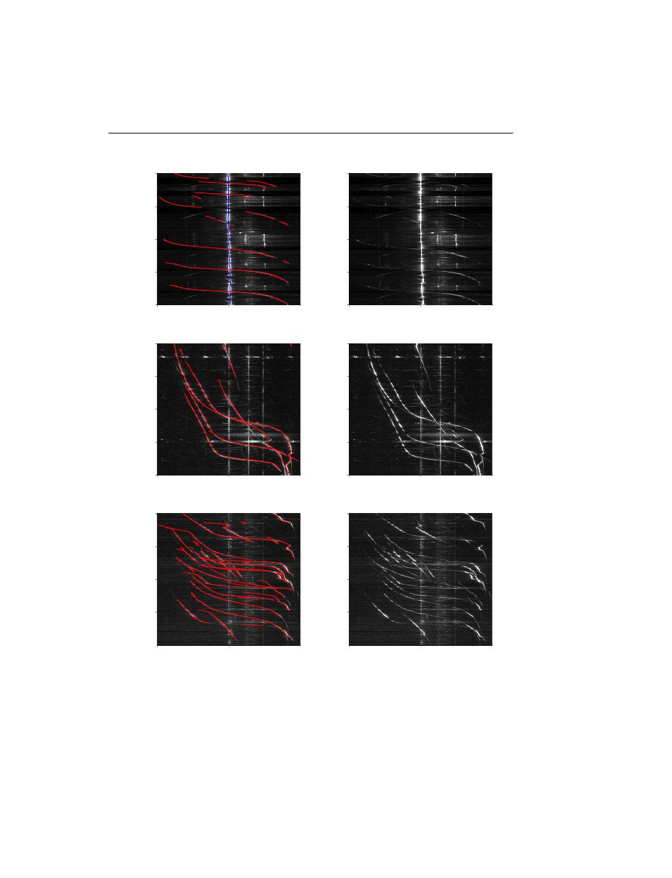
96
5. Instantaneous Doppler signature extraction
-84.9
49750000
+84.7
20:13:42
20:46:29
21:19:16
21:52:03
22:24:51
J
2
, 2012-07-11
-84.9
49750000
+84.7
20:13:42
20:46:29
21:19:16
21:52:03
22:24:51
J
2
, 2012-07-11
-84.9
49750000
+84.7
16:01:40
16:08:57
16:16:15
16:23:32
16:30:50
J
1
, 2014-04-01
-84.9
49750000
+84.7
16:01:40
16:08:57
16:16:15
16:23:32
16:30:50
J
1
, 2014-04-01
-84.9
49750000
+84.7
13:04:30
13:23:42
13:42:55
14:02:07
14:21:20
J
1
, 2014-04-04
-84.9
49750000
+84.7
13:04:30
13:23:42
13:42:55
14:02:07
14:21:20
J
1
, 2014-04-04
Figure 5.8: Left: Result of tracing spectrogram matrix S
I
, I = J
1
, J
2
; Right: Image before trac-
ing. Horizontal frequency axis are expressed in Hz, vertical in wall clock units of time while the
recording was taken.

5.5 Case Study
97
Examination of correlation values starts with the variable t
d
. The fact that it does not correlate with
any of the other parameters is an indicator of the stability of the system’s performance with respect
to the time time gap between signatures. It means that in the case of short time gaps the system
manages to extract signatures at the same level of performance as in the case of longer time gaps.
The linear relation between D
o
and D
e
describes the stability of the model’s performance measured
within different recording sessions. A significant linear relation between D
o
and FA and the value
of the fraction D
o
/FA which equals 1.95 indicate the stability of the selection technique used in the
model.
The relation between the detection rate D
e
/D
o
and the false alarm rate was found to equal −0.42
which indicates decrease in false alarm rate while increase in detected curves rate and vice versa.
It was found that there is no correlation between aSNR and any other parameter, which at that stage
of analysis is challenging to interpret.
Finally, there is a very significant correlation between the time t
e
and FA which confirms the linear-
ity of the model.
The efficiency of the system was found to equal D
e
/D
o
= 71 %.
5.5.2
Simulated signal
The tests in this subsection were conducted with simulated data introduced in 5.4.2. To check the
quality of signature extraction of the algorithm, the same parameter values presented in Table 5.1
that were used to test the real signal, were used.
Results presented in this section are based on 1400 simulations with varying parameters A
st
(x, y),
A
f i
(x, y), alt, V
c
, P
av
and randomly chosen statistical model. During each simulation the exact lo-
cation of Doppler signature on time-frequency plane was known based on (5.1). The exact Doppler
was then stored as (f
D
, a
o
, t), f
D
(t) , a
o
(t, f
D
), where t denotes time instances of Doppler signa-
ture, f
D
the frequency values and a
o
amplitude values (SNR dB). Moreover the extracted signatures
were stored in a form of (ω
l
, a
l
, t [st, en]), ω
l
(t) , a
l
(t, ω
l
) where t [st, en] denotes time instances
over which the extraction was successful, ω
l
the frequency values and a
l
amplitude values of the
extraction (SNR dB). The amplitude values of the extracted signature were averaged over time
t [st, en] so that each signature was indicated by its averaged SNR aSNR.
To compare the efficiency of the system on the set of statistical models the ratio r
e
between lengths of
extraction time t [st, en] and exact Doppler time length t was calculated as r
e
=
t[st,en]
t
. Dependency
of r
e
as a function of aSNR is shown in Fig. 5.10. Scattered values were fitted with a third order
polynomial (TOP) (red solid curves in Fig. 5.10) and compared for every model in Fig. 5.11 together
with the standard deviation of difference
σ
s
=
1
t (en) − t (st)
t[st,en]
[f
D
(t [st, en]) − ω
l
(t [st, en])]
2
(5.27)
The standard deviation values were fitted with third order polynomial for the Nonfluctuating and
Ogive models, the rest (Swerling 1-2) were equipped with fitted lines. Note that the scale of right
figure was changed for the Ogive curve ([0.638, 2.4]).
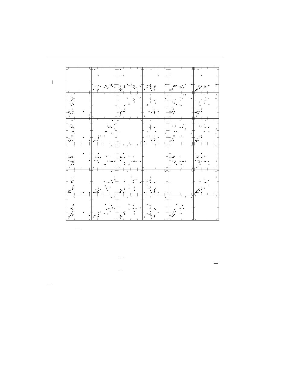
98
5. Instantaneous Doppler signature extraction
0
0.5
1
5
10
15
20
5
10
15
5
6
7
8
0
10
20
0
10 20 30
0
5
10
15
5 10 15 20
5 10 15
5 6 7 8 0
10
200
0.5
1
t
e
F
A
a
SNR
D
e
D
o
t
d
t
e
FA
aSNR
D
e
D
o
t
d
-0.13
-0.12
0.18
-0.09
0.11
-0.13
0.92
0.05
0.83
0.79
-0.12
0.92
-0.1
0.6
0.58
0.18
0.05
-0.1
0.22
0.28
-0.09
0.83
0.6
0.22
0.86
0.11
0.79
0.58
0.28
0.86
Figure 5.9: Pairwise correlation plot between variables presented in Table 5.2.
An overall performance of the system with simulated data can be expressed with an average value
of the parameter r
e
which was equal to r
e
= [0.82, 0.77, 0.81, 0.47] for Nonfluctuating, Swerling
1,2 and Ogive respectively. The averaged values of σ
s
for the aforementioned models were σ
s
=
[0.21, 0.23, 0.22, 0.74] Hz. The values of r
e
for three first models indicate a good performance of the
algorithm, but the relatively smaller value for the fourth one is caused by the fact that an Ogive was
detectable mainly when the case (5.26b) was in use (π − 2ϕ < β < π). Average standard deviation
σ
s
values do not exceed a frequency resolution in time-frequency plane which equals ∼ 0.91 Hz.
It is worth noting that the algorithm is able to separate between two or more intersecting signals
– the system recognizes them and follows the curves separately, as illustrated in Fig. 5.12, which
in that respect is an advantage over an algorithm presented in Djurovi´c and Stankovi´c (2004). The
experiment with two targets was conducted under the same conditions as defined earlier in section
5.4.2 with transmitting power P
av
= 25 W which resulted in aSNR = 5.39 dB. The intersection
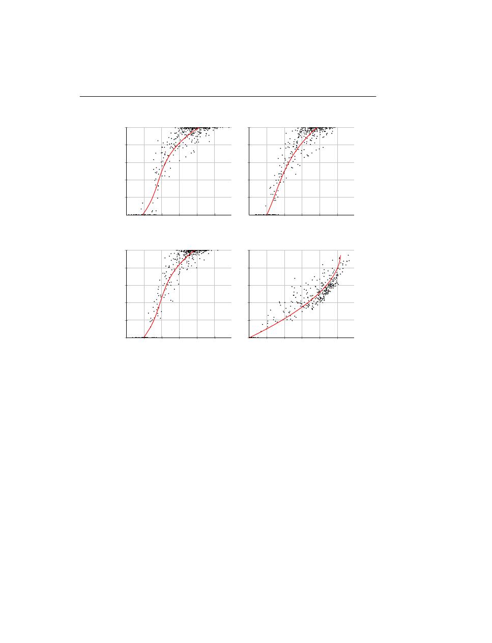
5.6 Discussion
99
0
2
4
6
8
10
0
0.2
0.4
0.6
0.8
1
r
e
Nonfluctuating
0
2
4
6
8
10
0
0.2
0.4
0.6
0.8
1
Swerling 1
0
2
4
6
8
10
0
0.2
0.4
0.6
0.8
1
aSNR dB
r
e
Swerling 2
0
2
4
6
8
10
0
0.2
0.4
0.6
0.8
1
aSNR dB
Ogive
Figure 5.10: Extraction time to exact Doppler time ratio r
e
as a function of aSNR (averaged SNR
over extracted time length t [st, en]) for three statistical models and an ogive.
does not influence the quality of extraction frequency-wise and there is no significant alternation of
trend of σ
s
, see right illustration in Fig. 5.12.
5.6
Discussion
This work is devoted to establishing a novel method of instantaneous Doppler signature extraction
from within Very High Frequency (VHF) band spectrogram images. We establish a Probability
Density Function (PDF) of the First Order Derivative of Doppler Shift (FODDS). This PDF is used
for estimating the expected value and therefore the expected frequency shift. The structure of the
mathematical model consists of a number of blocks, the most relevant of which are:
• A Cell Averaging – Constant False Alarm Rate (CA-CFAR) block responsible for detection
of amplitude-wise outlying cells;
• Construction of pretenders based on Center of Mass (CoM) formulae;
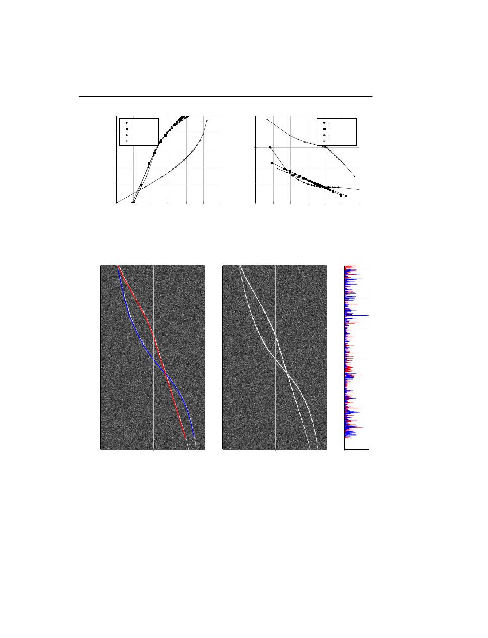
100
5. Instantaneous Doppler signature extraction
0
2
4
6
8
10
0
0.2
0.4
0.6
0.8
1
aSNR dB
r
e
Nonfluctuating
Swerling 1
Swerling 2
Ogive
0
2
4
6
8
10
0
0.2
0.4
0.638
2.4
aSNR dB
σ
s
Nonfluctuating
Swerling 1
Swerling 2
Ogive
Figure 5.11: Ratio r
e
as a function of aSNR (left figure) and standard deviation of difference
f
D
(t [st, en]) − ω
l
(t [st, en]) as a function of aSNR (right right). Note change of scale for Ogive
model [0.638, 2.4].
-83.1
49750000
+81.5
03:20
06:40
10:00
13:20
16:40
20:00
ω Hz
-83.1
49750000
+81.5
ω Hz
0
2.27
σ
s
Hz
Figure 5.12: Extraction of two targets. Left: extracted features; center: simulated spectrogram;
right: standard deviation of frequency differences σ
s
between extracted signatures and exact signa-
tures. Vertical axes represent wall clock time [MM:SS].
.

5.6 Discussion
101
• Classification of pretenders which uses signal energy concentration and frequency difference
between two consecutive steps and PDF of FODDS;
• The case of intersection of multiple signals is solved by predicting the signals’ location in the
frequency domain;
• A block of combining signals is responsible for linking two signals into one across a time
gap between them and a distance gap between their predicted frequency values. The missing
link is then created by extrapolating with a second order polynomial based on the number of
points from the proper ends of the both signals.
Based on twenty one recording sessions that were tested with the technique developed in this paper
we observed a 73 % efficiency in extracting Doppler signatures, while in the case of the synthetic
signal an efficiency of [0.82,0.77,0.81,0.47] was achieved for Nonlinear, Swerling 1, 2 and Ogive
test signals, respectively. This fact, combined with the possibility in which many more transmitter -
receiver pairs are used, may establish a system like the one described in Ptak et al. (2014) with which
hopefully no civilian large aircraft is untraceable when the receivers work together in a multi-static
configuration.

102
5. Instantaneous Doppler signature extraction

C
HAPTER
VI
Aircraft classification based on bistatic radar cross section
The paper studies instantaneous Doppler signature extraction from within Very High Frequency
(VHF) band spectrogram presented by the authors in previous work Ptak et al. (2015). The context
of the current method is long-range aircraft detection by VHF Doppler effect. The method pro-
posed calculates Bistatic Radar Cross Section (BRCS) profiles and the correlation between them
for different types of aircraft. The analysis is based on data represented by Automatic Dependent
Surveillance - Broadcast (ADS-B) trajectory collection and Passive Bistatic Radar (PBR) with TV
station as an illuminator of opportunity. Throughout the analysis ADS-B data on location of an
aircraft was adjusted with the use of extracted Doppler shift information. This ground truth infor-
mation on location was then used for proper evaluation of BRCS profiles and finally validating the
extraction method. The method is able to classify common inter-continental aircraft by size class
with 70 % accuracy from a hundred kilometer distance using an illuminator of opportunity located
300 km away.
6.1
Introduction
The almost eighty years long history of Bistatic Radar (BR) demonstrates to us that this subject
has been resurged for a reason. With advanced technology and increasing computational power of
processors we are able to use more of the features given by BR systems. BR has been tested in a
number of military applications. To name a few of them: homing missile control, forward scatter
fences, multistatic radars.
In this and previous related work the authors have attempted to construct a cheap and easily ex-
ploitable method for tracking aircraft in a passive bistatic configuration. The strategy of using
Doppler-only information is introduced and tested in a real-life scenario in Ptak et al. (2014) (Chap-
ter 4). This method is further enhanced in Ptak et al. (2015) (Chapter 5) by developing a method for
instantaneous Doppler extraction from within spectrogram representation of Very High Frequency
(VHF)-band scattered signal. The method was tested for component detection in the spectrogram
in a long-range baseline scenario (301 km), as well as with numerous statistical methods including
Nonfluctuating, Swerling I and II and synthetic ogive models.
The scope of this paper is further elaboration of this extraction method. This time the model is used
for examination of Bistatic Radar Cross Section (BRCS) profiles for classification of aircraft.
103

104
6. Aircraft classification based on bistatic radar cross section
Recent publications related to the subject of BRCS include problems such as Instrument Landing
System (ILS) misguidance of landing-course aircraft by taxed large-sized aircraft Geise et al. (2008),
influence on plane electromagnetic wave reflection, and therefore BRCS, caused by radionuclide
coating on the aircraft’s surface with different atmospherical conditions Liu et al. (2015).
In Gente et al. (2012) authors studied BRCS profiles of Panavia 200 Tornado and a Lockheed F117
Nighthawk in THz time domain. The decimeter band used for both receiving and transmitting
photoconductive antennas on scaled models resulted in very accurate measurements of their profiles,
down to the precision of distinguishing aircraft equipped with bombs from the one without them.
In other studies (Pisane et al., 2014), (Pisane, 2013) a novel method for Non-Cooperative Target
Recognition (NCTR) based on BRCS and Automatic Dependent Surveillance - Broadcast (ADS-B)
information within Passive Bistatic Radar (PBR) configuration is developed. The authors success-
fully classified detected aircraft into two groups of large-size aircraft and mid-size aircraft. The
BRCS is evaluated with a test set of trajectories and then the metrics are applied to the BRCS for
each cell in aspect angle δ – bistatic angle β to construct a pattern for each size-group for each cell.
The analysis presented in the current work differs from the aforementioned contributions. First of
all it uses PBR of VHF band in a long distance tracking for about 330 km of aircraft’s trajectory
length. Secondly the method of extracting Doppler signature is independently evaluated aside from
the ADS-B based synthetic Doppler prior information that suggests approximate location of Doppler
shift on time-frequency plane. The approach presented here differs from Pisane et al. (2014) also
by the fact that we use proximity of trajectories as a grouping factor rather that aspect angle-bistatic
angle sectioning.
6.2
Data acquisition and preprocessing
This section describes the configuration of PBR used and preparation of the recorded data for further
analysis.
6.2.1
Acquisition
The Radio Signal Data (RSD) was obtained with use of 4-element horizontal dipole array, described
in 3.3.1. The location of the receiver is denoted with R in Fig. 6.1, however its configuration with
J
1
.
Saint Petersburg transmitter, denoted as T in Fig. 6.1, has transmitting frequency f
t
= 49.75 MHz
and Effective Radiated Power (ERP) of 149 kW. The receiver was located a distance of d
TR
=
301.8 km away from the transmitter. The receiving aerial is connected to a FT-100D receiver used
in CW/USB mode with 500 Hz filter. Coaxial feed line loss between aerial and receiver is about
3 dB. Audio from the receiver is connected to computer’s sound card for numerical analysis. The
required audio width for aircraft scatter doppler observations is less than ±100 Hz from the 600 Hz
center audio frequency. Because the audio center frequency is low and bandwidth is very narrow,
the 8-bit signal quality used for analysis is adequate.
Such preprocessed signal was then sent via internet with use of Ventrilo
TM
software with sampling
frequency of 8 kHz to location in Oslo, Norway. Average signal delay varied at around 79 ms.
The signal was then transformed using Short Time Fourier Transform (STFT) with adjusted width
of symmetrically positioned Hann window of L = 1 s and calculation time step of G = 0.5 s.
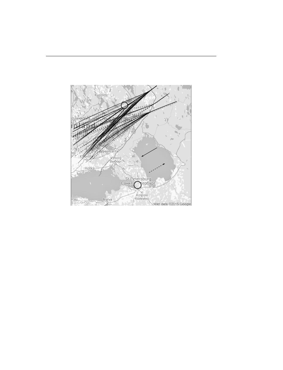
6.2 Data acquisition and preprocessing
105
This overlapped form of the spectrogram guarantees that the signal’s magnitude will be preserved
Izraelevitz (1985). Moreover in Chapter 5 authors stated that studies on First Order Derivative of
Doppler Shift (FODDS) ensure the choice of the window length being correctly adjusted.
J
T
e–w
w–e
Figure 6.1: Geographical location of transmitter T and receiver R and trajectories of FR24 data.
Solid and dashed lines correspond to east-west and west-east azimuths, respectively.
In parallel, yet another type of data FR24 was collected from flightradar24.com website. The FR24
data consists of tracks of aircraft in proximity to the the transmitter and the receiver. The tracks on
the other hand were built of the following most relevant columns of data: latitude, longitude, alti-
tude, aircraft type designator International Civil Aviation Organization (ICAO) and wall-clock time
of the sample being measured. The sample was collected in average every 5 s. During recordings
of FR24 ninety nine different trajectories created by eleven different types of aircraft were collected
from which seven most frequent types were used for the analysis, see Table 6.1. The trajectories are
depicted in Fig. 6.1.
6.2.2
Preprocessing
After the synchronous recordings of RSD and FR24 has been finished, the analysis of RSD for
tracing of Doppler and carrier signatures is started. The tracing of Doppler signature and carrier
was conducted using the technique presented in Chapter 5. The resulting data consists of vectors
of Doppler frequency ω
l
and the associated amplitude a
l
as a function of time t as well as carrier
frequency ω
c
and associated amplitude a
c
as a function of time t. For each extracted signature the

106
6. Aircraft classification based on bistatic radar cross section
Table 6.1: Types of aircraft together with ICAO designator, number of appearances grouped by
azimuth and basic specifications. The bullet sign indicates aircraft used in the analysis.
Number
Wing Number
of
area
of
Aircraft
ICAO trajectories
m
2
engines
e-w
w-e
• Airbus A330-300
A333
9
7
363.1
2
• Airbus A340-300
A343
13
2
363.1
4
• Airbus A340-600
A346
4
1
437
4
Boeing 737-800
B738
1
1
125
2
• Boeing 747-400
B744
7
5
541.2
4
• Boeing 777-200
B772
12
7
427.8
2
Boeing 777-200LR B77L
0
4
427.8
2
• Boeing 777-300ER B77W 16
5
427.8
2
• Boeing 787-8 Pax2 B788
3
1
325
2
Gulfstream V
GLF5
1
0
105.6
2
associated FR24 signature was found by calculating the proximity between the extracted Doppler
and the FR24-resulted Doppler on time-frequency plane.
The FR24-related Doppler signature was calculated based on spherical coordinates lat, lon and
altitude alt with respect to the location of the transmitter T and the receiver R by the following
formulae (6.1) and (6.2).
f
FR24
D
(t) =
f
t
c
d (d
TA
(t) + d
AR
(t))
dt
(6.1)
d
TA(AR)
(t) = 2R
E
(R
E
+ alt (t)) (1 − cos (ξ
TA
(AI))) + alt (t)
2
1
2
(6.2)
where R
E
= 6371 km is the mean radius of the Earth, ξ
TA
and ξ
AR
, correspond to great circle
arcs, measured in degrees and connecting the transmitter with the aircraft and the aircraft with the
receiver, respectively, c is the velocity of propagation of electromagnetic waves (light), d
TA
, d
AR
and d
TR
denote distances between transmitter and an aircraft, an aircraft and receiver and trans-
mitter and receiver, respectively. The angles were derived with use of Vincenty’s Inverse Formulae
(VIF) Vincenty (1975) (2.4) and based on the 1984 World Geodetic System (WGS84) spheroid.
Clarification of these notations is presented in Fig. 4.4.
Since the trajectory based on FR24’s latitude and longitude information was distorted, the resulting
Doppler frequency f
FR24
D
was distorted too, see yellow dots in Fig. 6.2. The noisy data is due to
asynchronous data collection by different ADS-B parties. This is caused most likely by differences
in PC clock time settings and partially by delay from the time when the Global Positioning Sys-
tem (GPS) measurement was taken on board of the aircraft to the time of reception with ADS-B
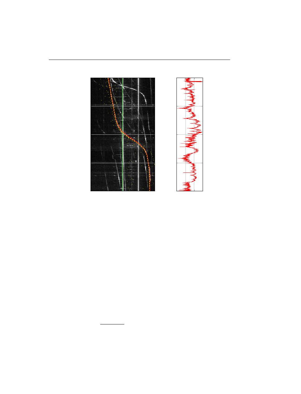
6.2 Data acquisition and preprocessing
107
-84.37
49750000
84.57
12:59:35
13:04:25
13:09:15
13:14:05
13:18:56
ω Hz
J
1
, 2014-09-16
-8.51 0
8
16
12:59:35
13:04:25
13:09:15
13:14:05
13:18:56
a
l
dB
Figure 6.2: Spectrogram: yellow dots - Doppler shift based on FR24 data f
FR24
D
, yellow dashed line
- smoothed Doppler shift based on FR24 data f
FR24
D
, red line - extracted Doppler curve ω
l
, green
line - extracted carrier ω
c
; Right: Amplitude of the extracted Doppler signature a
l
.
receiver. To compensate for this noise the data on latitude, longitude and altitude was transformed
from spherical to cartesian coordinates, then smoothed and interpolated with respect to time t. The
smoothing window was equal to 10 s and interpolation was chosen to match the time resolution of
RSD data G = 0.5 s. At the end the interpolated data was transformed back to spherical coordinates
and the Doppler frequency was calculated and denoted by f
FR24
D
, see yellow dashed line in Fig. 6.2.
Because the information on Doppler shift ω
l
was extracted from within the spectrogram, see red
line on the spectrogram in Fig. 6.2, it can now be used for further adjustment of the trajectory of
an aircraft. It is worth noting that the synthetic Doppler (FR24) projected onto the spectrogram do
not overlap with the extracted Doppler - there is a noticeable shift between them with respect to
time and the close-to-baseline region of FR24 signature is steeper than that of RSD, see Fig. 6.2.
The remedy for this difference was introduced by shifting the whole trajectory by latitude lat
sh
and
longitude lon
sh
factors and looking for the minimum cost function which is presented in (6.3).
f
cost
= f
FR24
D
− ω
l
f
D,max
f
D,max
+ |ω
l
|
(6.3)
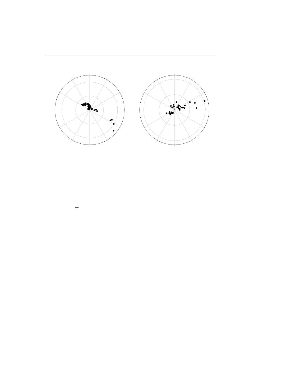
108
6. Aircraft classification based on bistatic radar cross section
0
30
60
90
120
150
180
210
240
270
300
330
0
10km
20km
e-w
0
30
60
90
120
150
180
210
240
270
300
330
0
4km
8km
w-e
Figure 6.3: Distribution of found latitude and longitude shifts lat
sh
, lon
sh
(azimuth, distance km)
for groups east-west (left) and west-east (right).
where f
D,max
denotes maximum achievable Doppler shift which is expressed by
f
D,max
= 2
f
t
c
V
c,max
.
(6.4)
In the case of maximum cruising velocity, V
c,max
is set to V
c,max
= 278 km h
−1
which yields
f
D,max
= 92 Hz. The proposed form of cost function intentionally puts higher weight onto the
region close-to-baseline-crossing to account for the shift in time between the signatures. The found
distribution of latitude and longitude shifts in polar coordinates is presented in Fig. 6.3. Most of
the trajectory shifts do not exceed a 5 km boundary. The curve distribution pattern in e-w group
would suggest that the needed shift was dictated not only by time delay but also by displacement in
spherical coordinates.
By this process RSD data was now also accompanied by FR24-based information like trajectory
(latitude lat , longitude lon and altitude alt), type of an aircraft ICAO and FR24-based Doppler
signature. This set of numbers can be denoted by
ω
l
, a
l
, ω
c
, a
c
, lat , lon , alt, f
FR24
D
(t). This
set can be further divided into two subsets, namely those azimuth-related to west-east (w-e) and
east-west (e-w). All of the analyses are taking into account the east-west group. Additionally the
remaining group of aircraft is categorized by their size into three groups: G1:mid-size (B788, A333,
A343), G2:large-size(B772, B77W, A346) and the largest aircraft G3:(B744).

6.3 Bistatic radar cross section comparison
109
6.3
Bistatic radar cross section comparison
The BRCS σ
B
of the extracted signatures was calculated using the following formulae (Proakis and
Salehi, 2007).
σ
B
=
a
l
a
c
(4π) d
2
TA
d
2
AR
d
2
TI
(6.5)
The equation (6.5) was derived from bistatic radar formulae (Willis, 2005) in (6.6)
a
l
=
P
av
G
T
G
R
λ
2
σ
B
(4π)
3
d
2
TA
d
2
AR
(6.6)
and direct-path link budget (6.7) for the receiver not being in line-of-sight from the transmitter
a
c
= P
av
G
T
G
R
L
S
(6.7)
where P
T
is the transmitter power output, G
T
is the transmitting antenna power gain, G
R
is the
receiving antenna power gain, λ is the wavelength, L
S
denotes free space path loss of the signal
between the transmitter and the receiver. No other losses are assumed. The free space loss factor
L
S
is expressed as
L
S
=
λ
4πd
TR
2
(6.8)
Therefore by substituting L
S
from (6.8) into (6.7), then dividing side-wise (6.7) and (6.6) and by
rearranging, the form in equation (6.5) is attained. The bistatic angle β is estimated from the location
of the aircraft, the transmitter and the receiver in order to represent the BRCS as a function of β.
Since the observed aircrafts’ trajectories were not overlapping each other (more than one air cor-
ridor was used) the subsequent analysis have been carried out under a trajectory proximity as-
sumption. The validity of this assumption is tested by analyzing trajectories pair-wise, taking into
account the average spatial distance between them that should be relatively small. In the case
when trajectories are located in the immediate neighborhood of the receiver, the propagation of the
bounced signal is no longer classified as a two-dimensional case, but as a three dimensional one,
and proximity is judged accordingly. An average distance between two trajectories tr
i
and tr
j
is
derived by taking every point of these two sequences tr
i
(k
1
) = (lat
i
(k
1
) , lon
i
(k
1
)) , k
1
= 1...n
1
,
tr
j
(k
2
) = (lat
j
(k
2
) , lon
j
(k
2
)) , k
2
= 1...n
2
and solving equation 6.9.
d (tr
i
, tr
j
) = 0.5
1
n
2
n
2
k
2
=1
min
k
1
∈[1,n
1
]
d (tr
i
(k
1
) , tr
j
(k
2
))
+
1
n
1
n
1
k
1
=1
min
k
2
∈[1,n
2
]
d (tr
i
(k
1
) , tr
j
(k
2
))
(6.9)
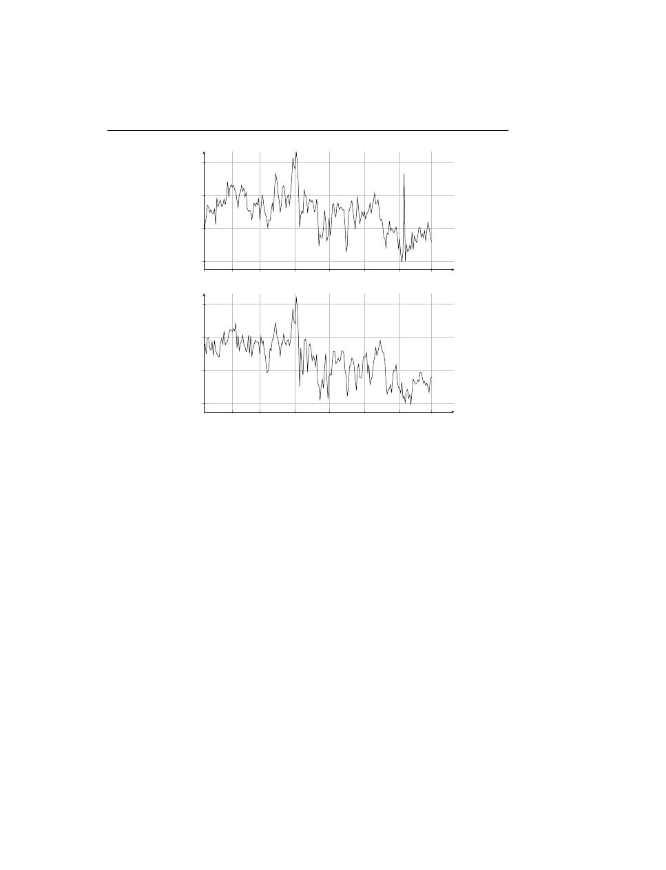
110
6. Aircraft classification based on bistatic radar cross section
-130
-90
-50
0
50
100
150
196
−20
−10
0
10
A333
a
l
/a
c
dB
-130
-90
-50
0
50
100
150
196
−20
−10
0
10
A333
distance km
a
l
/a
c
dB
Figure 6.4: Fraction of the reflected to direct signal from two Airbus A330-300 aircrafts in time
domain.
where d (tr
i
(k
1
) , tr
j
(k
2
)) is an averaged distance between tr
i
(k
1
) and tr
j
(k
2
). Flight trajectory
pairs were screened for an arbitrarily chosen maximal minimum distance d
min
= 10 km that had
to be attained between the trajectories. This screening resulted in 618 pairs of trajectories being
selected for further analysis out of the 2145 available at the beginning.
Fig. 6.4 depicts a difference in amplitude fraction of the extracted Doppler signal and the extracted
carrier signal for two aircraft of type A333’s in distance domain. The distance domain describes
distance from an aircraft to the baseline, negative for approaching part and positive for departing
part. In this example a correlation between signals reached ρ
A
= 0.92 while the average distance
between trajectories equaled d (tr
i
, tr
j
) = 0.52 km.
As it was mentioned earlier the performance of the technique presented in Ptak et al. (2015) ought
to be tested by checking the correlation between calculated BRCS’s for different types of aircraft.
This is achieved by calculating the correlation between BRCS for every pair of trajectories available,
then classifying them by the aircraft group and finally calculating an average correlation factor. The
result of this analysis is presented in Table 6.2.
We can notice the relatively higher correlation factors of the three groups on the diagonal of the
matrix. In the next analysis we have found an optimal correlation threshold for which the number
of aircraft-pairs from the same class is maximized and the pairs from different classes is minimized.
The threshold has been found to be equal 0.58. The result for this is shown in Fig. 6.5.
6.3 Bistatic radar cross section comparison
111
Table 6.2: An average correlation with respect to the group of an aircraft.
ICAO B788 A333 A343 B772 B77W A346 B744
B788
0.57
0.65
0.56
0.28
0.20
0.28
0.20
A333
0.65
0.74
0.65
0.31
0.35
0.41
0.24
A343
0.56
0.65
0.70
0.36
0.42
0.34
0.29
B772
0.28
0.31
0.36
0.75
0.73
0.69
0.35
B77W 0.20
0.35
0.42
0.73
0.76
0.71
0.36
A346
0.28
0.41
0.34
0.69
0.71
0.80
0.38
B744
0.20
0.24
0.29
0.35
0.36
0.38
0.75
G
1
:B
78
8,
A3
33
,
A3
43
G
2
:B
77
2,
B
77
W
,
A3
46
G
3
:B
74
4
G1
:B788, A333, A343
G2
:B772, B77W, A346
G3
:B744
group/aircraft type
gr
ou
p
/ai
rc
raf
t
ty
p
e
G1:B788,A333,A343
G2:B772,B77W,A346
G3:B744
G1
:B788,A333,A343
G2
:B772,B77W
,A346
G3
:B744
group:aircraft type
group:aircraft
type
Figure 6.5: Result of optimal correlation-threshold estimation. Red squares denotes values over the
threshold, black ones values below the threshold.
The number of correctly classified pairs within groups on the diagonal significantly exceed the
number of misclassified pairs. With this condition in mind the probability of misdetection/detection
was calculated and presented in Table 6.3. The values on the diagonal reflect the probability of
correct classification, whereas the upper and lower triangles the probability of misclassification.

112
6. Aircraft classification based on bistatic radar cross section
Table 6.3: Probability of classification/misclassification between the groups G1, G2 and G3.
aircraft group
G1: B788, A333, A343 G2: B772, B77W, A346 G3: B744
G1
74
101
= 0.73
34
171
= 0.19
4
59
= 0.06
G2
34
171
= 0.19
162
205
= 0.79
12
75
= 0.16
G3
4
59
= 0.06
12
75
= 0.16
5
7
= 0.71
6.4
Discussion
The paper validates the performance of the mathematical model of instantaneous Doppler signature
extraction from within Very High Frequency (VHF) band spectrogram image (Chapter 5) by com-
paring Bistatic Radar Cross Section (BRCS) profiles of seven types of aircraft. Firstly the Flight
Radar 24 (FR24) and Radio Signal Data (RSD) data was acquired from which the latter was prepro-
cessed using Short Time Fourier Transform (STFT). Then with the technique presented in (Chap-
ter 5) Doppler and carrier signatures were estimated. In parallel the FR24 data was enhanced by
smoothing and interpolating trajectories in order to de-noise the data. Additionally, with the use of
the extracted Doppler shift information the FR24 trajectories were shifted to minimize the frequency
distance between FR24 and RSD Doppler shifts. Then the BRCS for each Doppler amplitude a
l
and
associated carrier amplitude a
c
and trajectory (lat ,lon ) was calculated. Because of different air
corridors used by recorded aircraft, further analysis of BRCS comparison was conducted with re-
spect to the distance between trajectories. The correlation between BRCS’s was calculated for each
pair of trajectories for which the average distance do not exceed 10 km. The resulting matrix of cor-
relations, especially diagonal values, between different groups of the aircraft validates the extraction
technique as well as the data acquisition and preprocessing methods, as does the further examination
of classification performance by means of thresholding the correlation in order to estimate optimal
classification to misclassification ratio.

B
IBLIOGRAPHY
Alfonzetti, S., Borzi, G., Jul 2000. A fast method for computation of the bistatic radar cross section.
Magnetics, IEEE Transactions on 36 (4), 921–924.
Allen, J., Rabiner, L., nov. 1977. A unified approach to short-time Fourier analysis and synthesis.
Proceedings of the IEEE 65 (11), 1558 – 1564.
Auger, F., Flandrin, P., Lin, Y.-T., McLaughlin, S., Meignen, S., Oberlin, T., Wu, H.-T., Nov 2013.
Time-Frequency Reassignment and Synchrosqueezing: An Overview. Signal Processing Maga-
zine, IEEE 30 (6), 32–41.
Bailey, J., Gray, G., Willis, N., Nov 1977. Sanctuary Signal Processing Requirements. In: Circuits,
Systems and Computers, 1977. Conference Record. 1977 11th Asilomar Conference on. pp. 310–
315.
Baldauf, J., Lee, S.-W., Lin, L., Jeng, S.-K., Scarborough, S., Yu, C., Sep 1991. High frequency
scattering from trihedral corner reflectors and other benchmark targets: SBR versus experiment.
Antennas and Propagation, IEEE Transactions on 39 (9), 1345–1351.
Bhattacharyya, A. K., 4 1991. Radar Cross Section Analysis and Control (Artech House Radar
Library). Artech Print on Demand.
Bracewell, R., 2000. The Fourier Transform and Its Applications. Electrical engineering series.
McGraw Hill.
Brown, J., Woodbridge, K., Griffiths, H., Stove, A., Watts, S., 2012a. Passive bistatic radar exper-
iments from an airborne platform. Aerospace and Electronic Systems Magazine, IEEE 27 (11),
50–55.
Brown, J., Woodbridge, K., Stove, A., Watts, S., 2010. Air target detection using airborne passive
bistatic radar. Electronics Letters 46 (20), 1396–1397.
Brown, J., Woodbridge, K., Stove, A., Watts, S., 2012b. VHF airborne passive bistatic radar ground
clutter investigation. In: Radar Systems (Radar 2012), IET International Conference on. pp. 1–5.
Canny, J., nov. 1986. A Computational Approach to Edge Detection. Pattern Analysis and Machine
Intelligence, IEEE Transactions on PAMI-8 (6), 679 –698.
Carr, J., Hippisley, G., 2011. Practical Antenna Handbook 5/e. McGraw-Hill Education.
Carrier, G. F., Krook, M., Pearson, C. E., 7 2005. Functions of a Complex Variable: Theory and
Technique (Classics in Applied Mathematics). Society for Industrial & Applied.
113

114
Bibliography
Chutatape, O., Guo, L., 1999. A modified Hough transform for line detection and its performance.
Pattern Recognition 32 (2), 181 – 192.
Clemente, C., Soraghan, J., January 2014. GNSS-Based Passive Bistatic Radar for Micro-Doppler
Analysis of Helicopter Rotor Blades. Aerospace and Electronic Systems, IEEE Transactions on
50 (1), 491–500.
Cohen, L., Jul 1989. Time-frequency distributions-a review. Proceedings of the IEEE 77 (7), 941–
981.
Coifman, R., Rokhlin, V., Wandzura, S., June 1993. The fast multipole method for the wave equa-
tion: a pedestrian prescription. Antennas and Propagation Magazine, IEEE 35 (3), 7–12.
Daubechies, I., Maes, S., 4 1996. Wavelets in Medicine and Biology, 1st Edition. CRC Press, Ch.
A Nonlinear Squeezing of the Continuous Wavelet Transform Based on Auditory Nerve Models,
pp. 527–546.
Department of Transportation, Federal Aviation Administration, 2 2009. Extended Squitter Auto-
matic Dependent Surveillance - Broadcast (ADS-B) and Traffic Information Service - Broadcast
(TIS-B) Equipment Operating on the Radio Frequency of 1090 Megahertz (MHz). Tech. rep.,
Federal Aviation Administration.
Djurovi´c, I., Stankovi´c, L., 2004. An algorithm for the Wigner distribution based instantaneous
frequency estimation in a high noise environment. Signal Processing 84 (3), 631 – 643.
URL
http://www.sciencedirect.com/science/article/pii/
S0165168403003463
Doughty, S. R., 2008. Development and Performance Evaluation of a Multistatic Radar System.
Ph.D. thesis, University of London.
Driedger, J., Muller, M., Ewert, S., Jan 2014. Improving Time-Scale Modification of Music Signals
Using Harmonic-Percussive Separation. Signal Processing Letters, IEEE 21 (1), 105–109.
Dubois, C., Davy, M., May 2007. Joint Detection and Tracking of Time-Varying Harmonic Com-
ponents: A Flexible Bayesian Approach. Audio, Speech, and Language Processing, IEEE Trans-
actions on 15 (4), 1283–1295.
Durak, L., Arikan, O., May 2003. Short-time Fourier transform: two fundamental properties and an
optimal implementation. Signal Processing, IEEE Transactions on 51 (5), 1231–1242.
Farina, A., 2005. Knowledge-Based Radar Signal and Data Processing. RTO Educational Notes.
RTO/NATO, Ch. Introduction to Radar Signal & Data Processing: The Opportunity, pp. 1–24.
Ferguson, B., Oct 1996. Time-frequency signal analysis of hydrophone data. Oceanic Engineering,
IEEE Journal of 21 (4), 537–544.
Filloux, J. H., Forbes, A. J., Harrison, G. A., Langel, R. A., Malin, S., 2 1987. Geomagnetism,
Volume 1. Academic Press.
Fogle, O., Rigling, B., 2012. Micro-Range/Micro-Doppler Decomposition of Human Radar Signa-
tures. Aerospace and Electronic Systems, IEEE Transactions on 48 (4), 3058–3072.

115
Geise, R., Enders, A., Vahle, H., Spieker, H., Aug 2008. Scaled Measurements of Instrument-
Landing-System Disturbances Due to Large Taxiing Aircraft. Electromagnetic Compatibility,
IEEE Transactions on 50 (3), 485–490.
Gente, R., Jansen, C., Geise, R., Peters, O., Gente, M., Krumbholz, N., Moller, C., Busch, S.,
Koch, M., July 2012. Scaled Bistatic Radar Cross Section Measurements of Aircraft With a Fiber-
Coupled THz Time-Domain Spectrometer. Terahertz Science and Technology, IEEE Transactions
on 2 (4), 424–431.
Georgescu, R., Willett, P., 2012. RFS MCMC Predetection Fusion Applied to Multistatic Sonar
Data. Aerospace and Electronic Systems, IEEE Transactions on 48 (4), 2894–2907.
Griffiths, H., Sept 2010. Multistatic, MIMO and networked radar: The future of radar sensors? In:
Radar Conference (EuRAD), 2010 European. pp. 81–84.
Griffiths, H., Baker, C., June 2005. Passive coherent location radar systems. Part 1: performance
prediction. Radar, Sonar and Navigation, IEE Proceedings - 152 (3), 153–159.
Gürel, L., Bagci, H., Castelli, J. C., Cheraly, A., Tardivel, F., 2003. Validation through comparison:
Measurement and calculation of the bistatic radar cross section of a stealth target. Radio Science
38 (3), n/a–n/a.
Hara, S., Wannasarnmaytha, A., Tsuchida, Y., Morinaga, N., Aug 1997. A novel FSK demodula-
tion method using short-time DFT analysis for LEO satellite communication systems. Vehicular
Technology, IEEE Transactions on 46 (3), 625–633.
Hlawatsch, F., Boudreaux-Bartels, G., April 1992. Linear and quadratic time-frequency signal rep-
resentations. Signal Processing Magazine, IEEE 9 (2), 21–67.
Howland, P., 1995. Passive Tracking Of Airborne Targets Using Only Doppler And Doa Informa-
tion. In: Algorithms for Target Tracking, IEE Colloquium on. pp. 37–39.
Howland, P., 1999. Target tracking using television-based bistatic radar. Radar, Sonar and Naviga-
tion, IEE Proceedings - 146 (3), 166–174.
hua QIN, D., fa WANG, B., 2002. Bistatic {RCS} Prediction with Graphical Electromagnetic Com-
puting (GRECO) Method for Moving Targets. Chinese Journal of Aeronautics 15 (3), 161 – 165.
ICAO, 2006. Airborne Collision Avoidance System (ACAS) Manual. International Civil Aviation
Organization, 999 University Street, Montréal, Quebec, Canada H3C 5H7, 1st Edition.
ICAO, 2008. Technical Provisions for Mode S Services and Extended Squitter. International Civil
Aviation Organization, 999 University Street, Montréal, Quebec, Canada H3C 5H7, 1st Edition.
ICAO, April 2012. Aircraft Type Designators. International Civil Aviation Organization, 999 Uni-
versity Street, Montréal, Quebec, Canada H3C 5H7, 1st Edition.
IEEE, 1990. IEEE Standard Radar Definitions. IEEE Std 686-1990.
IEEE Standard (521
TM
), 2003. IEEE Standard Letter Designations for Radar-Frequency Bands.
IEEE Std 521-2002 (Revision of IEEE Std 521-1984).

116
Bibliography
Izraelevitz, D., Dec 1985. Some results on the time-frequency sampling of the short-time Fourier
transform magnitude. Acoustics, Speech and Signal Processing, IEEE Transactions on 33 (6),
1611–1613.
Jackson, J., Rigling, B., Moses, R., April 2010. Canonical Scattering Feature Models for 3D and
Bistatic SAR. Aerospace and Electronic Systems, IEEE Transactions on 46 (2), 525–541.
Karney, C. F., 2013. Algorithms for geodesics. Journal of Geodesy 87, 43–55.
Kell, R., Aug 1965. On the derivation of bistatic RCS from monostatic measurements. Proceedings
of the IEEE 53 (8), 983–988.
Khan, N., Boashash, B., Feb 2013. Instantaneous Frequency Estimation of Multicomponent Nonsta-
tionary Signals Using Multiview Time-Frequency Distributions Based on the Adaptive Fractional
Spectrogram. Signal Processing Letters, IEEE 20 (2), 157–160.
Kuschel, H., Heckenbach, J., Muller, S., Appel, R., 2008. On the potentials of passive, multistatic,
low frequency radars to counter stealth and detect low flying targets. In: Radar Conference, 2008.
RADAR ’08. IEEE. pp. 1–6.
Kwok, H., Jones, D., Oct 2000. Improved instantaneous frequency estimation using an adaptive
short-time Fourier transform. Signal Processing, IEEE Transactions on 48 (10), 2964–2972.
Lane, T., Alexander, N., Blevins, C., 1999. The bistatic coherent measurement system (BICOMS).
In: Radar Conference, 1999. The Record of the 1999 IEEE. pp. 154–159.
Li, J., Phung, S. L., Tivive, F., Bouzerdoum, A., June 2012. Automatic classification of human
motions using Doppler radar. In: Neural Networks (IJCNN), The 2012 International Joint Con-
ference on. pp. 1–6.
Li, X.-F., Xie, Y.-J., Yang, R., 2009. BISTATIC RCS PREDICTION FOR COMPLEX TARGETS
USING MODIFIED CURRENT MARCHING TECHNIQUE. PIER 93, 13–28.
Liu, K., Dec 1993. Novel parallel architectures for short-time Fourier transform. Circuits and Sys-
tems II: Analog and Digital Signal Processing, IEEE Transactions on 40 (12), 786–790.
Liu, W., Zhu, J., Cui, C., Wang, X., Zhang, S., Zhang, R., Tang, T., Huang, Y., Huang, R., Jan 2015.
The Influence of Plasma Induced by alpha -Particles on the Radar Echoes. Plasma Science, IEEE
Transactions on 43 (1), 405–413.
Malanowski, M., Kulpa, K., Kulpa, J., Samczynski, P., Misiurewicz, J., February 2014. Analysis of
detection range of FM-based passive radar. Radar, Sonar Navigation, IET 8 (2), 153–159.
Malanowski, M., Kulpa, K., Samczynski, P., Misiurewicz, J., Kulpa, J., 2012. Long range FM-based
passive radar. In: Radar Systems (Radar 2012), IET International Conference on. pp. 1–4.
Matsuo, M., Yuba, Y., Yamane, K., Jan 1970. Bistatic radar cross-section measurements by pendu-
lum method. Antennas and Propagation, IEEE Transactions on 18 (1), 83–88.
Mixon, D., 2012. Doppler-Only Multistatic Radar. Biblioscholar.

117
Ochiai, H., Nov 2004. A novel trellis-shaping design with both peak and average power reduction
for OFDM systems. Communications, IEEE Transactions on 52 (11), 1916–1926.
Oppenheim, A. V., Schafer, R. W., 8 2009. Discrete-Time Signal Processing (3rd Edition) (Prentice
Hall Signal Processing), 3rd Edition. Prentice Hall.
Pan, X.-Y., Wang, W., Liu, J., Ma, L., Feng, D.-J., Wang, G.-Y., December 2013. Modulation
effect and inverse synthetic aperture radar imaging of rotationally symmetric ballistic targets with
precession. Radar, Sonar Navigation, IET 7 (9), 950–958.
Peterson, A. M., Teague, C. C., Tyler, G. L., Oct 1970. Bistatic-radar observation of long-period,
directional ocean-wave spectra with loran a. Science 170 (3954), 158–161.
Pielemeier, W., Wakefield, G., Simoni, M., Sep 1996. Time-frequency analysis of musical signals.
Proceedings of the IEEE 84 (9), 1216–1230.
Pisane, J., 1 2013. Automatic target recognition using passive bistatic radar signals. Ph.D. thesis,
University of Liège and SUPELEC.
Pisane, J., Azarian, S., Lesturgie, M., Verly, J., January 2014. Automatic Target Recognition for
Passive Radar. Aerospace and Electronic Systems, IEEE Transactions on 50 (1), 371–392.
Plante, F., Meyer, G., Ainsworth, W., May 1998. Improvement of speech spectrogram accuracy by
the method of reassignment. Speech and Audio Processing, IEEE Transactions on 6 (3), 282–287.
Proakis, J., Salehi, M., 2007. Digital Communications, 5th Edition. McGraw-Hill higher education.
McGraw-Hill Education.
Ptak, P., Hartikka, J., Ritola, M., Kauranne, T., July 2014. Long-distance multistatic aircraft tracking
with VHF frequency doppler effect. Aerospace and Electronic Systems, IEEE Transactions on
50 (3), 2242–2252.
Ptak, P., Hartikka, J., Ritola, M., Kauranne, T., Submitted in January 2015. Instantaneous Doppler
signature extraction from within a spectrogram image of a VHF band. Aerospace and Electronic
Systems, IEEE Transactions on.
Rokhlin, V., 1990. Rapid solution of integral equations of scattering theory in two dimensions.
Journal of Computational Physics 86 (2), 414 – 439.
Rothwell, E., Chen, K., Nyquist, D., Sep 1998. An adaptive-window-width short-time Fourier trans-
form for visualization of radar target substructure resonances. Antennas and Propagation, IEEE
Transactions on 46 (9), 1393–1395.
Russell, S. J., Norvig, P., 1 1995. Artificial Intelligence: A Modern Approach, 1st Edition. Prentice
Hall.
Schetne, K., Mount, W., Aug 1965. Full-scale bistatic radar cross-section measurement method.
Proceedings of the IEEE 53 (8), 1083–1084.
Siegel, K., Alperin, H., Bonkowski, R., Crispin, J., Maffett, A., Schensted, C., Schensted, I., Mar
1955. Bistatic Radar Cross Sections of Surfaces of Revolution. Journal of Applied Physics 26 (3),
297–305.

118
Bibliography
Skolnik, M., 2003. Introduction to Radar Systems. McGraw-Hill.
Skolnik, M., 2008. Radar Handbook, Third Edition. Electronics electrical engineering. McGraw-
Hill Education.
Song, J., Lu, C.-C., Chew, W. C., Oct 1997. Multilevel fast multipole algorithm for electromagnetic
scattering by large complex objects. Antennas and Propagation, IEEE Transactions on 45 (10),
1488–1493.
Special Committee 186, 6 2002. Minimum Aviation System Performance Standards For Automatic
Dependent Surveillance Broadcast (ADS-B). Tech. rep., Radio Technical Commission for Aero-
nautics.
Straw, R., Cebik, L., Hallidy, D., Jansson, D., 2007. The ARRL Antenna Book, 21st Edition. ARRL
ANTENNA BOOK. ARRL.
Suberviola, I., Mayordomo, I., Mendizabal, J., Jan 2012. Experimental Results of Air Target Detec-
tion With a GPS Forward-Scattering Radar. Geoscience and Remote Sensing Letters, IEEE 9 (1),
47–51.
Szóstka, J., 2006. Fale i anteny. Wydawnictwa Komunikacji i Ł ˛
aczno´sci.
Thayaparan, T., Kennedy, S., Feb 2004. Detection of a manoeuvring air target in sea-clutter us-
ing joint time-frequency analysis techniques. Radar, Sonar and Navigation, IEE Proceedings -
151 (1), 19–30.
Thompson, E., Mar 1989. Bistatic radar noncooperative illumination synchronization techniques.
In: Radar Conference, 1989., Proceedings of the 1989 IEEE National. pp. 29–34.
Vincenty, T., 1975. Direct and inverse solutions of geodesics on the ellipsoid with application of
nested equations. Survey Review 22 (176), 88–93.
Weiland, T., 1996. Time Domain Electromagnetic Field Computation With Finite Difference Meth-
ods. International Journal of Numerical Modelling: Electronic Networks, Devices and Fields
9 (4), 295–319.
Willis, N., Griffiths, H., July 2008. Advances in bistatic radar (Willis, N.J. and Griffiths, H.D., Eds.;
2007) [Book Review]. Aerospace and Electronic Systems Magazine, IEEE 23 (7), 46–46.
Willis, N. J., 12 2005. Bistatic Radar, 2nd Edition. SciTech Publishing.
Wu, M., Dai, X., Zhang, Y., Davidson, B., Amin, M., Zhang, J., Sept 2013. Fall Detection Based
on Sequential Modeling of Radar Signal Time-Frequency Features. In: Healthcare Informatics
(ICHI), 2013 IEEE International Conference on. pp. 169–174.
Wu, P., Li, M., oct 1996. A novel Hough transform for curve detection. In: Systems, Man, and
Cybernetics, 1996., IEEE International Conference on. Vol. 4. pp. 2722 –2727 vol.4.
Xiangwei, M., Jian, G., You, H., Sept 2003. CFAR techniques for over-the-horizon radar. In: Intel-
ligent Signal Processing, 2003 IEEE International Symposium on. pp. 83–85.
Zebker, H. A., Tyler, G. L., Jan 1984. Thickness of Saturn’s Rings Inferred from Voyager 1 Obser-
vations of Microwave Scatter. Science 223 (4634), 396–398.

ACTA UNIVERSITATIS LAPPEENRANTAENSIS
609. PIRTTILÄ, MIIA. The cycle times of working capital: financial value chain analysis method.
2014. Diss.
610. SUIKKANEN, HEIKKI. Application and development of numerical methods for the mod-
elling of innovative gas cooled fission reactors. 2014. Diss.
611. LI, MING. Stiffness based trajectory planning and feedforward based vibration suppression
control of parallel robot machines. 2014. Diss.
612. KOKKONEN, KIRSI. From entrepreneurial opportunities to successful business networks -
evidence from bioenergy. 2014. Diss.
613. MAIJANEN-KYLÄHEIKO, PÄIVI. Pursuit of change versus organizational inertia: a study
on strategic renewal in the Finnish broadcasting company. 2014. Diss.
614. MBALAWATA, ISAMBI SAILON. Adaptive Markov chain Monte Carlo and Bayesian filter-
ing for state space models. 2014. Diss.
615. UUSITALO, ANTTI. Working fluid selection and design of small-scale waste heat recovery
systems based on organic rankine cycles. 2014. Diss.
616. METSO, SARI. A multimethod examination of contributors to successful on-the-job learning
of vocational students. 2014. Diss.
617. SIITONEN, JANI. Advanced analysis and design methods for preparative chromatographic
separation processes. 2014. Diss.
618. VIHAVAINEN, JUHANI. VVER-440 thermal hydraulics as computer code validation chal-
lenge. 2014. Diss.
619. AHONEN, PASI. Between memory and strategy: media discourse analysis of an industrial
shutdown. 2014. Diss.
620. MWANGA, GASPER GODSON. Mathematical modeling and optimal control of malaria.
2014. Diss.
621. PELTOLA, PETTERI. Analysis and modelling of chemical looping combustion process with
and without oxygen uncoupling. 2014. Diss.
622. NISKANEN, VILLE. Radio-frequency-based measurement methods for bearing current anal-
ysis in induction motors. 2014. Diss.
623. HYVÄRINEN, MARKO. Ultraviolet light protection and weathering properties of wood-
polypropylene composites. 2014. Diss.
624. RANTANEN, NOORA. The family as a collective owner - identifying performance factors in
listed companies. 2014. Diss.
625. VÄNSKÄ, MIKKO. Defining the keyhole modes - the effects on the molten pool behavior
and the weld geometry in high power laser welding of stainless steels. 2014. Diss.

626. KORPELA, KARI. Value of information logistics integration in digital business ecosystem.
2014. Diss.
627. GRUDINSCHI, DANIELA. Strategic management of value networks: how to create value in
cross-sector collaboration and partnerships. 2014. Diss.
628. SKLYAROVA, ANASTASIA. Hyperfine interactions in the new Fe-based superconducting
structures and related magnetic phases. 2015. Diss.
629. SEMKEN, R. SCOTT. Lightweight, liquid-cooled, direct-drive generator for high-power wind
turbines: motivation, concept, and performance. 2015. Diss.
630. LUOSTARINEN, LAURI. Novel virtual environment and real-time simulation based methods
for improving life-cycle efficiency of non-road mobile machinery. 2015. Diss.
631. ERKKILÄ, ANNA-LEENA. Hygro-elasto-plastic behavior of planar orthotropic material.
2015. Diss.
632. KOLOSENI, DAVID. Differential evolution based classification with pool of distances and
aggregation operators. 2015. Diss.
633. KARVONEN, VESA. Identification of characteristics for successful university-company part-
nership development. 2015. Diss.
634. KIVYIRO, PENDO. Foreign direct investment, clean development mechanism, and environ-
mental management: a case of Sub-Saharan Africa. 2015. Diss.
635. SANKALA, ARTO. Modular double-cascade converter. 2015. Diss.
636. NIKOLAEVA, MARINA. Improving the fire retardancy of extruded/coextruded wood-plastic
composites. 2015. Diss.
637. ABDEL WAHED, MAHMOUD. Geochemistry and water quality of Lake Qarun, Egypt.
2015. Diss.
638. PETROV, ILYA. Cost reduction of permanent magnet synchronous machines. 2015. Diss.
639. ZHANG, YUNFAN. Modification of photocatalyst with enhanced photocalytic activity for
water treatment. 2015. Diss.
640. RATAVA, JUHO. Modelling cutting states in rough turning of 34CrNiMo6 steel. 2015. Diss.
641. MAYDANNIK, PHILIPP. Roll-to-roll atomic layer deposition process for flexible electronics
applications. 2015. Diss.
642. SETH, FRANK. Empirical studies on software quality construction: Exploring human factors
and organizational influences. 2015. Diss.
643. SMITH, AARON. New methods for controlling twin configurations and characterizing twin
boundaries in 5M Ni-Mn-Ga for the development of applications. 2015. Diss.
644. NIKKU, MARKKU. Three-dimensional modeling of biomass fuel flow in a circulating flu-
idized bed furnace. 2015. Diss.
645. HENTTU, VILLE. Improving cost-efficiency and reducing environmental impacts of inter-
modal transportation with dry port concept - major rail transport corridor in Baltic Sea region.
2015. Diss.
646. HAN, BING. Influence of multi-phase phenomena on semibatch crystallization processes of
aqueous solutions. 2015. Diss.

Document Outline